Seeing beyond the bands
Where hyperspectral analysis diverges from multispectral — and what that divergence reveals about a crop. Measured on real scenes.

Francis Doumet
Co-Founder & CEO
For two decades, NDVI has been the default lens on crop health from orbit. It is fast, cheap, and everywhere — but it is also a single smoothed number, and that number hides more than most growers realize. This is a field note about what a continuous spectrum sees that a handful of broad bands cannot, worked through two real scenes rather than a lab bench.
The baseline · NDVI
The limits of a vegetation index
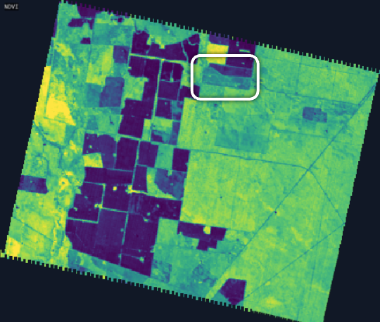
NDVI reads the contrast between the near-infrared light plants reflect and the red light they absorb — a reliable proxy for canopy vigour. But it returns a single smoothed signal, and three structural blind spots come with it.
Saturation
Once a canopy is dense enough, NDVI stops climbing even as the plant keeps changing — it flattens out past LAI (Leaf Area Index) > 3.
Thriving and over-mature fields read the same.
Blind to dry matter
NDVI uses only Red and NIR. Non-photosynthetic vegetation needs the SWIR, so dried and senescent material never registers.
Dry stalks look like bare soil.
Soil interference
In sparse, early-stage crops the soil background bleeds into the pixel and skews the index up or down.
Emergence looks healthier — or more stressed — than it is.
Resolution · sampling
Sparse bands vs. a continuous spectrum
The root cause is how the two sensor classes sample light. Multispectral instruments read a handful of broad points across 400–2500 nm; hyperspectral reads the same range as a near-continuous curve. The features that separate healthy from stressed sit between a multispectral sensor's bands — in wavelength ranges it never samples.

The evidence · two scenes
Two scenes, real reflectance
Everything that follows is measured over the same fields. We start from the multispectral baseline, then show what only the full spectrum resolves — no synthetic data, no lab spectra.
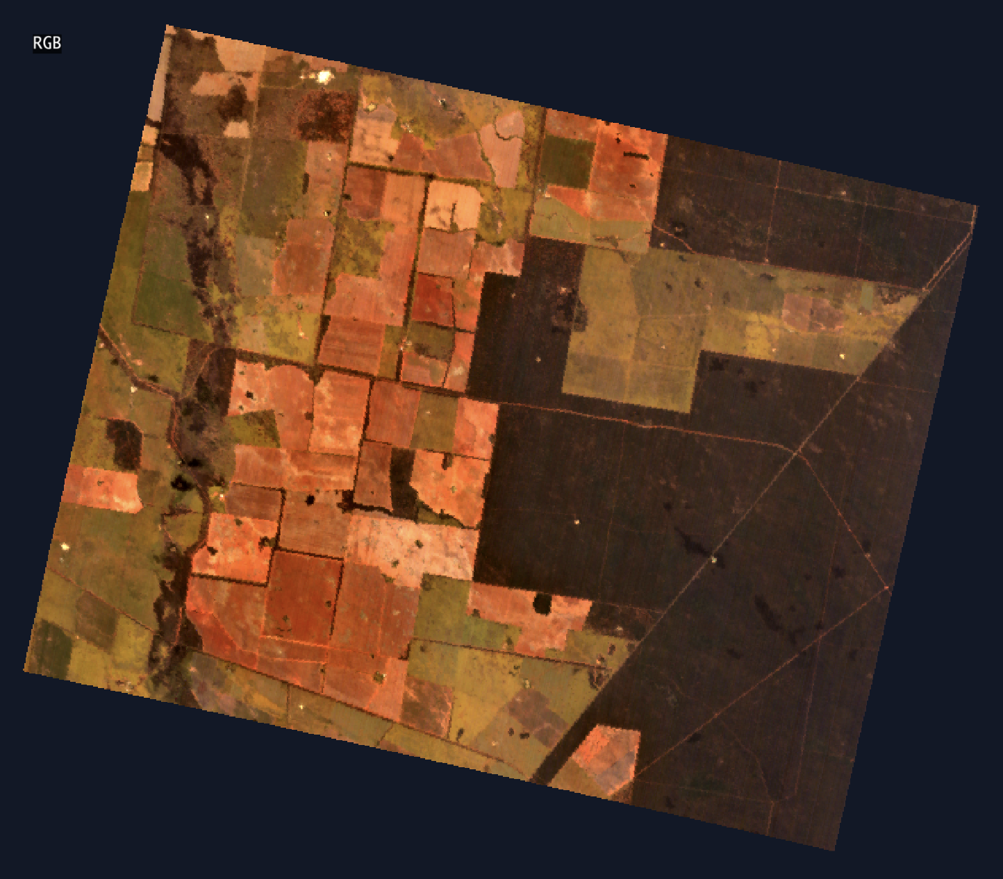
Pilinga, Australia
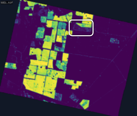
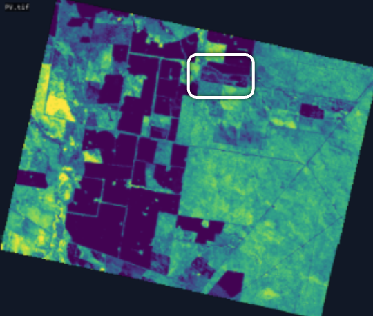
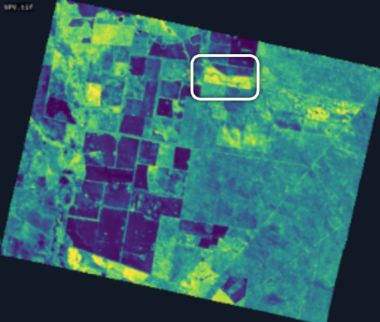
Planet Tanager · hyperspectralCropland and forest. Some fields harvested to bare soil, others holding green (PV) or dried (NPV) vegetation.
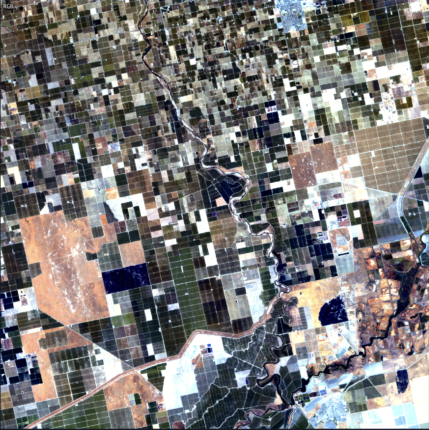
Central Valley, California
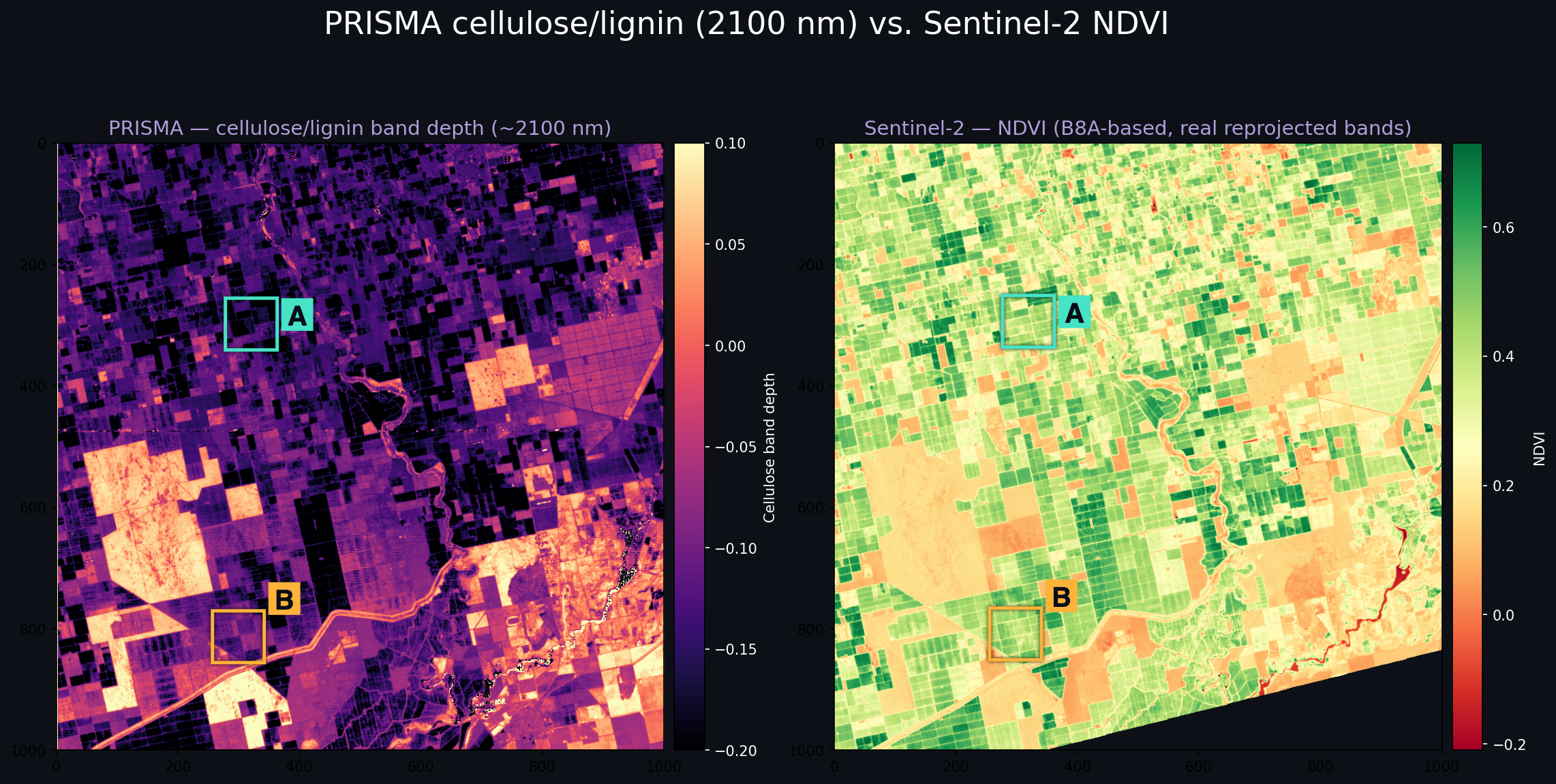
PRISMA vs Sentinel-2 · 7 days apartA dense agricultural mosaic along the delta — crops, fallow ground and water that the two sensor classes read very differently.
Tanager · unmixing
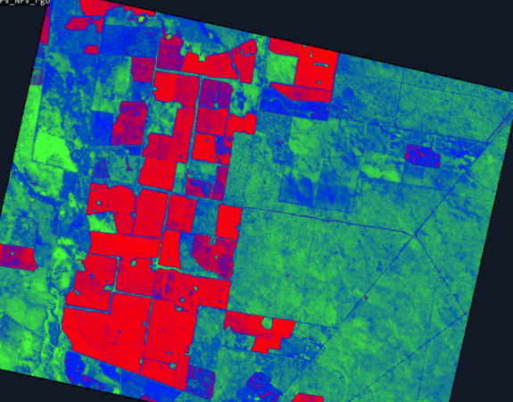
One index vs. three endmembers
Here is the core idea. NDVI gives one blended score per pixel — soil, weeds and crop averaged together, like a smoothie. Unmixing decomposes that same pixel back into the fraction that is Soil, PV (live vegetation) and NPV (dried, non-photosynthetic matter). Each layer becomes its own field-health signal.
Tanager · the NPV advantage
The dry-matter blind spot
Non-photosynthetic vegetation — dry branches, senescent leaves, crop residue — absorbs in the shortwave infrared near 2,100 and 2,300 nm from cellulose and lignin. Most multispectral sensors have broad SWIR bands, or none at all.
To a multispectral sensor, a field of dry corn stalks looks almost identical to bare brown dirt.
In-season, high NPV signals premature senescence from drought or disease.
Post-harvest, high NPV means crop residue protecting soil and sequestering carbon.
PRISMA · Feature 02 · dry matter
Same green, different chemistry
Dry plant material — cellulose, lignin, crop residue — absorbs near 2,100 nm in the shortwave infrared. Hyperspectral measures that band depth directly. Two fields can sit at the same high NDVI yet differ sharply in chemistry — one a lush vegetative canopy, the other already accumulating cellulose and lignin as it matures or carries residue.
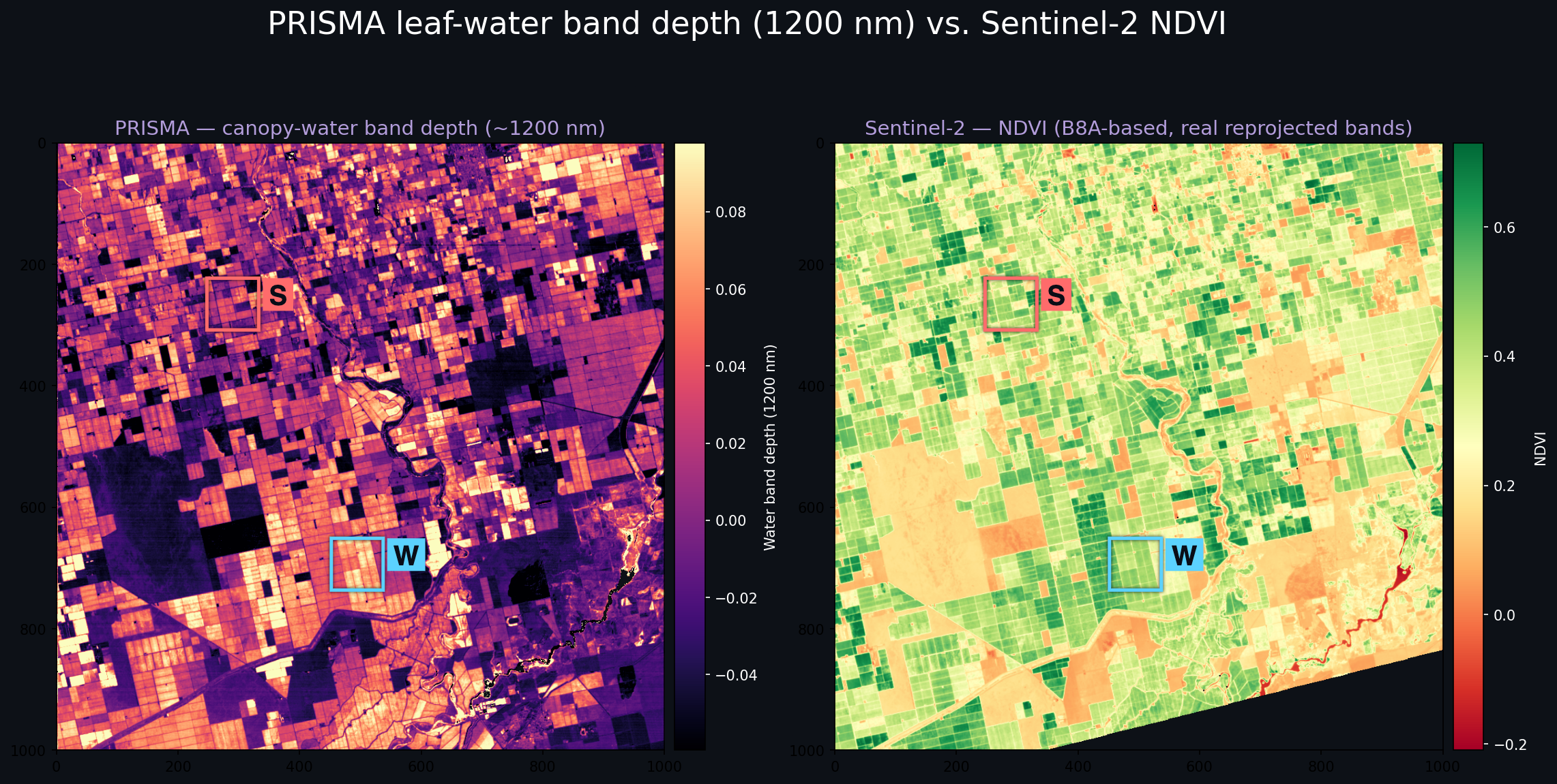
PRISMA · canopy water · 1200 nm
Green canopy, hidden water stress
Liquid water in a canopy produces a broad absorption near 1,200 nm. Hyperspectral measures its band depth directly — a true optical reading of how much water the leaves actually hold. Neighbouring fields, ostensibly the same crop, separate cleanly by hydration state — a distinction that looks identical in an NDVI image.
NDVI reports how green and dense a canopy is — not how much water it holds. The 1,200 nm absorption separates a canopy that is green-but-water-stressed from one that is green-and-well-watered. For irrigation, that is the difference between reacting after vigour drops and intervening while the canopy still looks healthy.
PRISMA · Feature 03 · the spectral gap
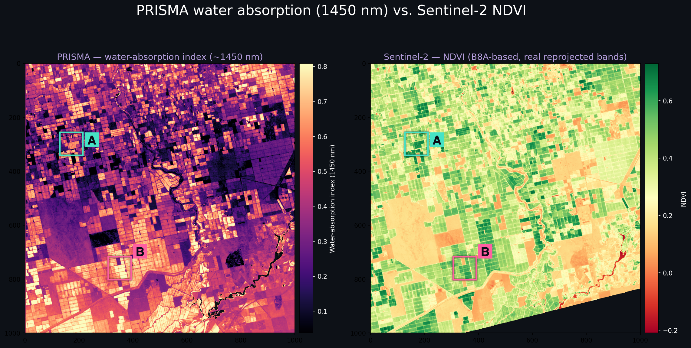
Where Sentinel-2 goes dark
The 1,450 nm water absorption sits squarely in a Sentinel-2 spectral gap — no band between 1375 nm (B10) and 1610 nm (B11). Hyperspectral reads it directly.
Not "hyperspectral does it better." Sentinel-2 cannot do it at all.
Read alongside the 1,200 nm map, this is a second, independent water window — two absorption features agreeing is harder to fool. And it keeps resolving water status where NDVI saturates across a closed canopy.
PRISMA · head-to-head · red edge
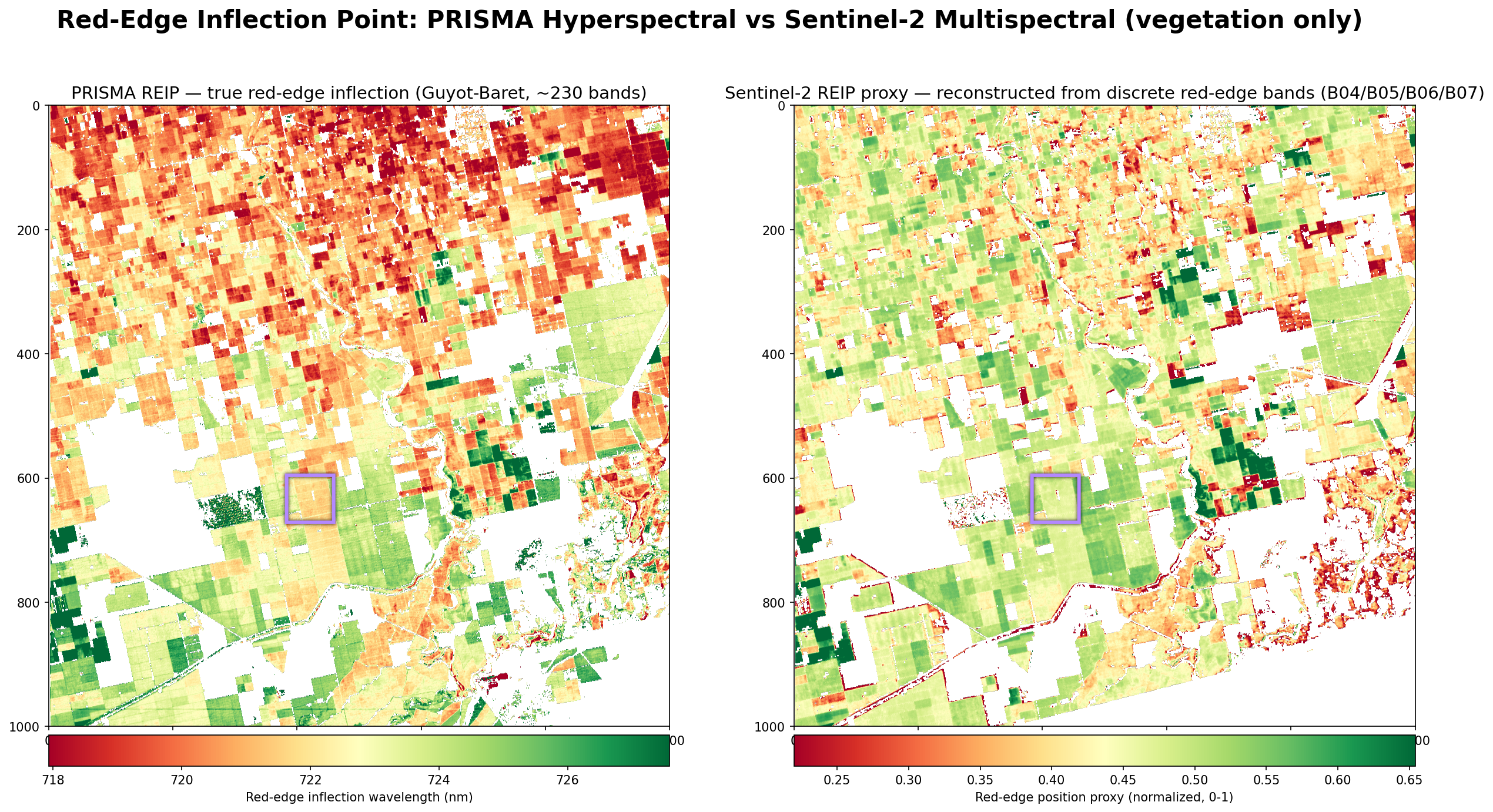
True wavelength vs. relative proxy
Hyperspectral resolves the red-edge inflection as a true wavelength — an actual position in nanometres (vegetation mean ≈ 722 nm), with smooth field-by-field gradients.
Sentinel-2's multispectral proxy can say "more shift than the neighbour" — not where the inflection sits.
The inflection wavelength tracks chlorophyll and nitrogen. As pigment builds, the red edge shifts to longer wavelengths (a healthy, N-rich canopy); as it drops, the edge slides back to shorter wavelengths — early stress, weeks before any visible yellowing.
Because hyperspectral gives an absolute wavelength reading, it can be checked against an agronomic threshold across dates and fields — the basis for variable-rate fertigation. Sentinel-2's relative proxy re-anchors every scene, so it can rank fields but never trigger a threshold.
less chlorophyll · stressed Higher λ ≈ 730 nm
more chlorophyll · healthy
Side by side
Multispectral vs. hyperspectral
Material Intelligence
From divergence to decision
By unmixing what multispectral blends together, hyperspectral turns crop colour into crop chemistry — a triple-threat field-health read.
From the pure PV fraction — without soil interference.
From the NPV fraction — organic matter returning to the soil.
From the soil fraction — tillage intensity and moisture effects.
Material Intelligence. Operationalized.
Clarity operationalizes hyperspectral and multispectral imagery into explainable, real-time material intelligence — from a conveyor belt to low-Earth orbit.
Related Resources
More product thinking and reference material from the Metaspectral team.
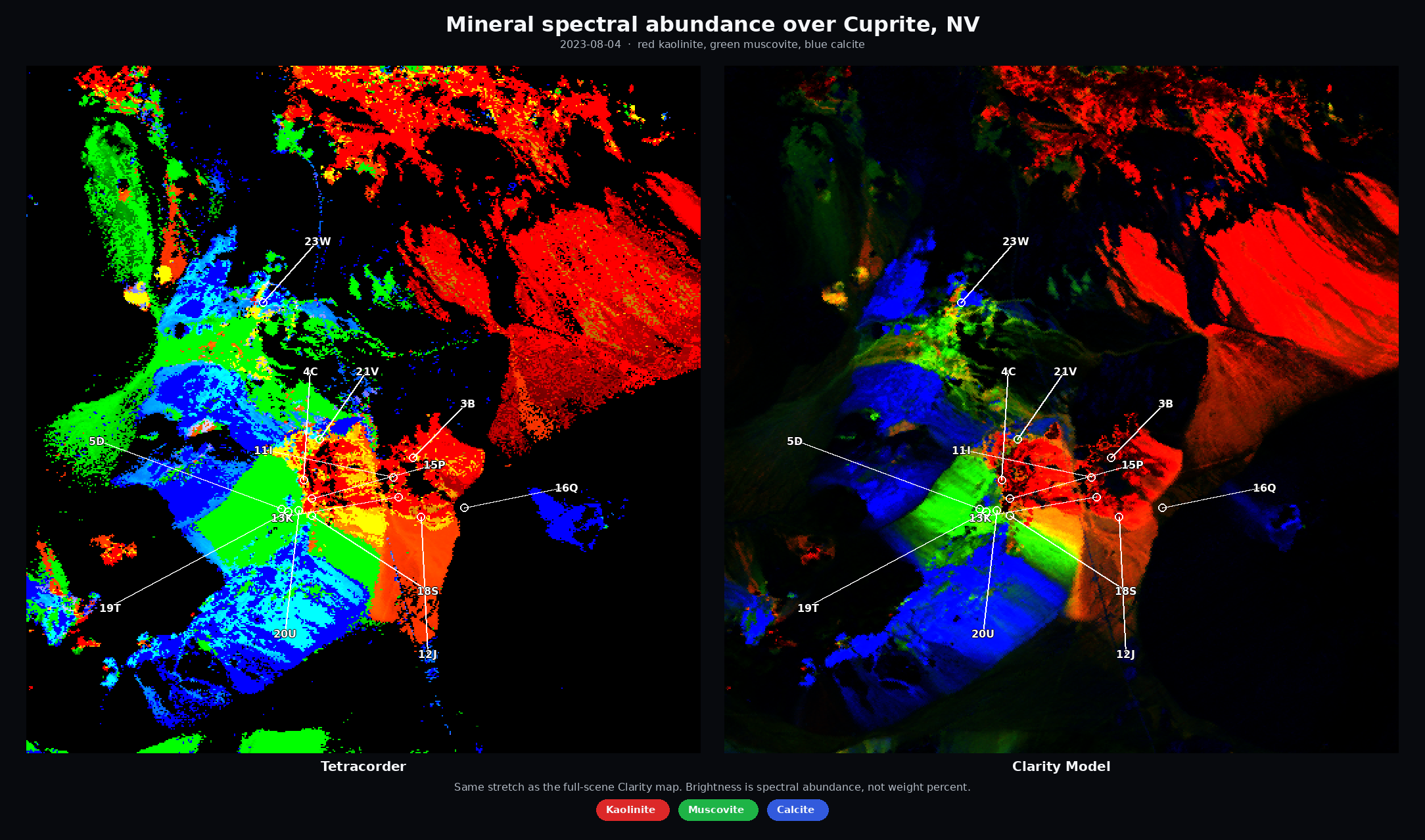
From Spectral Libraries to Cuprite — Better, Faster Alteration Maps
Exploration teams looking for copper, gold, and critical-mineral deposits use hyperspectral imagery to map exposed alteration and indicator minerals—clays, micas, iron oxides, carbonates, and related assemblages.
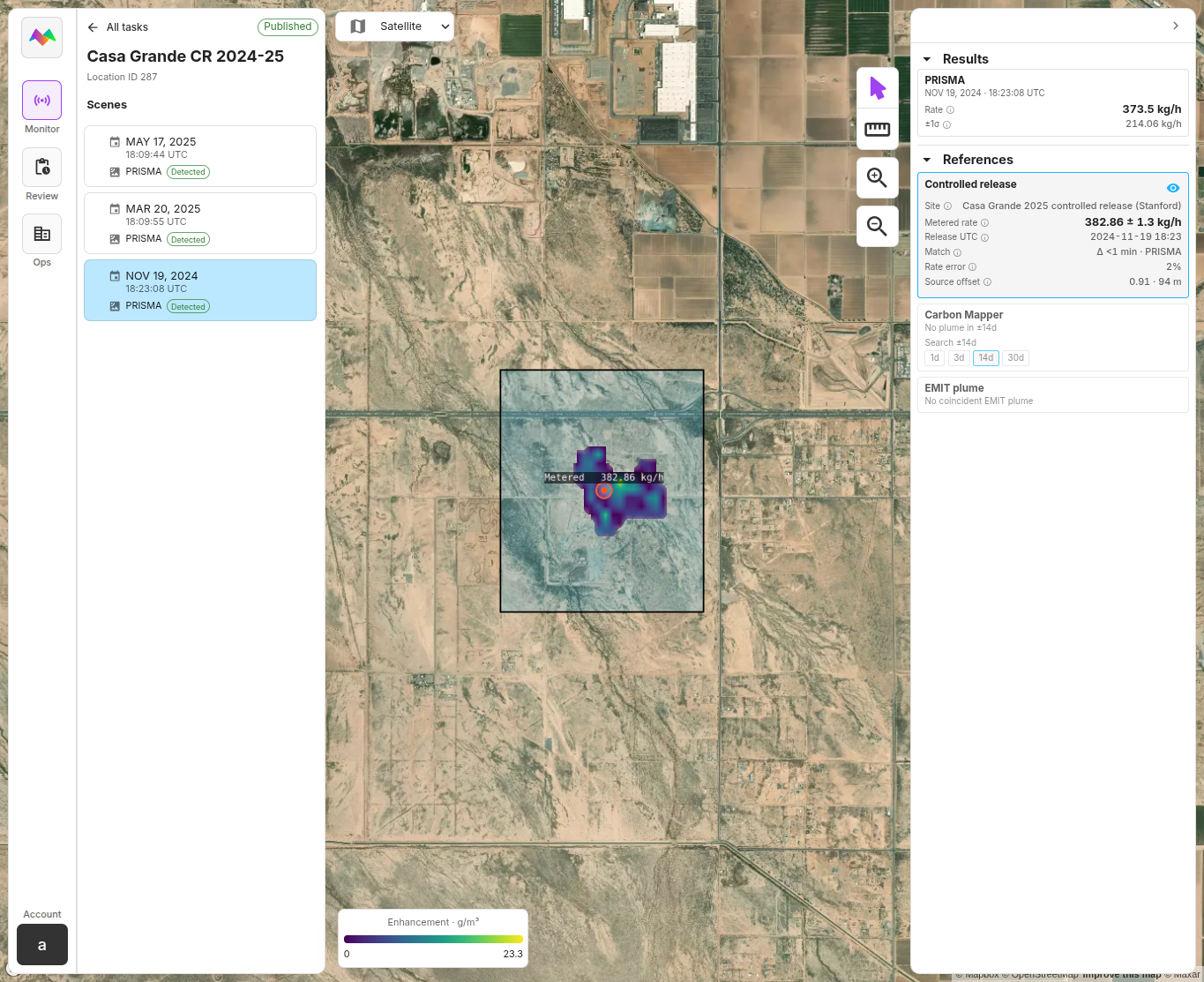
Clarity Plume™ Matches Metered Methane — Review It Faster, on Your Site
A controlled-release evaluation of Clarity Plume's production methane retrievals against PRISMA and EMIT, with metered releases, no-release periods, and review references beside the result.
Metaspectral Partners with Planet to Deliver Trusted Spectral Intelligence from Tanager Hyperspectral Data
Metaspectral announced its partnership with Planet Labs PBC to deliver trusted, evidence-based spectral intelligence from Planet Tanager™ hyperspectral data through Metaspectral Clarity.