Evaluating Deep Learning Spectral Unmixing From Pure Reference Spectra
A deep learning model trained only on synthetic mixtures — generated from pure reference spectra — outperforms classical solvers on four- and five-material mixtures across nine sensors. The benchmark: 325 real clay powder mixtures measured by lab spectrometers, pushbroom cameras, snapshot cameras, MWIR, and RGB.

Ahmed Sigiuk
Senior Deep Learning Engineer
Spectral unmixing answers a more useful question than simple classification: not only what material is present, but how much of each material is present.
That matters because real samples are rarely clean. A pixel can contain several minerals, coatings, contaminants, soils, plastics, or plant materials at once. In those cases, assigning one label to the whole pixel loses the information the sensor was meant to capture.
The practical challenge is training. Real mixtures with known proportions are difficult to collect at scale. Pure reference spectra are much easier to measure and maintain. In this study, we evaluate whether a deep learning (DL) model can start from those pure spectra, generate synthetic training mixtures, and then perform well on real measured mixtures.
The clearest result appears as the number of materials increases (Table 5, Figure 2). Classical methods are strong on simple two-material mixtures. By four- and five-material mixtures, the DL model beats the best classical solver on every sensor we tested.
Benchmark Dataset
We used the public multisensor intimate-mixture benchmark (Table 1). It is a useful test case because the same physical mixtures were measured by several instruments, while the ground-truth material proportions remain the same. That lets us compare methods across sensors without changing the underlying samples.
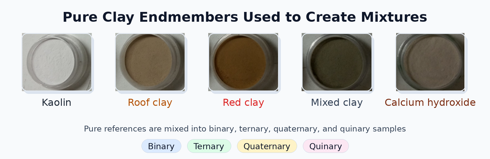
The mixtures are made from five clay-related endmembers: Kaolin, Roof clay, Red clay, Mixed clay, and Calcium hydroxide. Each real mixture has known mass-fraction abundances, so the evaluation measures how close each method gets to the true proportions. The clay spectra intentionally overlap, especially across the clay materials, but they also contain useful separation in overall spectral shape and in absorption regions around 1400 nm, 1900 nm, and 2100-2500 nm (Figure 1).
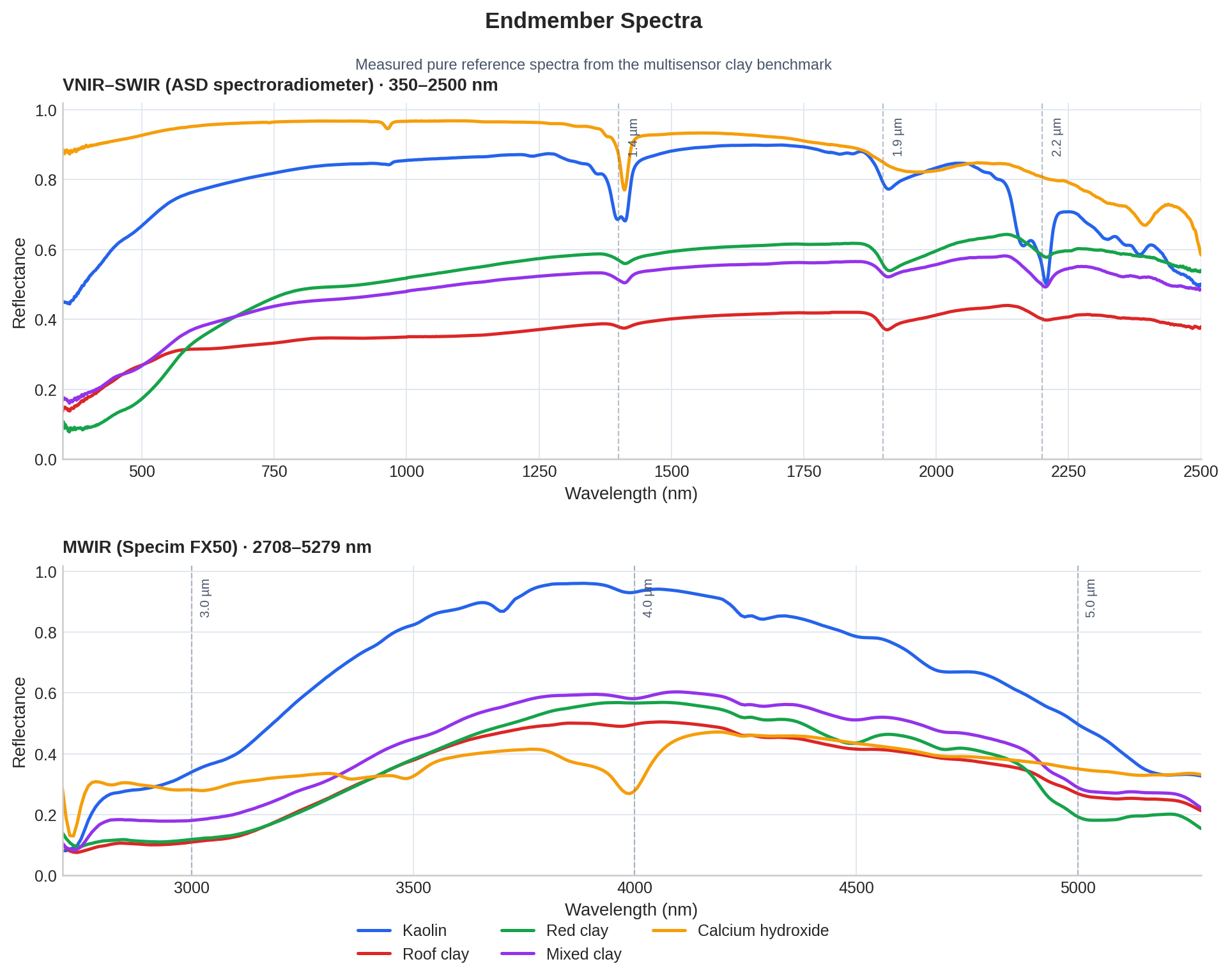
Figure 1. Measured pure endmember spectra: VNIR–SWIR from the ASD spectroradiometer (350–2500 nm) and MWIR from the Specim FX50 (2708–5279 nm).
| Item | Description |
|---|---|
| Dataset | Multisensor intimate-mixture benchmark |
| Real mixture samples | 325 measured mixtures, plus pure reference spectra |
| Endmembers | Kaolin, Roof clay, Red clay, Mixed clay, Calcium hydroxide |
| Evaluation target | Predict the abundance of each endmember in each real mixture |
Table 1. Summary of the benchmark dataset used for evaluation.
The 325 real mixtures are split by the number of materials present in each sample (Table 2):
| Mixture order | Meaning | Samples |
|---|---|---|
| Binary (k=2) | Two materials present | 60 |
| Ternary (k=3) | Three materials present | 150 |
| Quaternary (k=4) | Four materials present | 100 |
| Quinary (k=5) | Five materials present | 15 |
Table 2. Breakdown of real mixture samples by mixture order.
The full benchmark includes 13 sensors across visible, near-infrared, short-wave infrared, mid-wave infrared, and long-wave infrared ranges. Our experiments use the nine sensors in Table 3, spanning lab spectrometers, pushbroom cameras, snapshot cameras, MWIR, VNIR, SWIR, and RGB:
| Sensor | Bands | Range (nm) | Type / region |
|---|---|---|---|
| ASD spectroradiometer | 2151 | 350–2500 | Point spectrometer, VNIR-SWIR |
| PSR-3500 | 1024 | 345–2504 | Point spectrometer, VNIR-SWIR |
| Specim AisaFenix | 450 | 378–2504 | Pushbroom camera, VNIR-SWIR |
| Specim FX50 | 308 | 2708–5279 | MWIR camera |
| Specim sCMOS | 238 | 398–1001 | Pushbroom camera, VNIR |
| Cubert Ultris X20P | 164 | 350–1002 | Snapshot camera, VNIR |
| IMEC | 100 | 1120–1675 | Snapshot camera, SWIR |
| Senops HSC2 | 50 | 500–900 | Snapshot camera, VNIR |
| JAI RGB | 3 | 440–630 | RGB camera |
Table 3. The nine sensors used in our experiments.
Modeling Approach
Both the DL model and the classical baselines start from the same reference information: the five pure endmember spectra. What differs is how each one uses mixing methods. The DL model uses a mixing function only during training, both to generate synthetic data and inside the loss objective that reconstructs the mixed spectrum from predicted abundances, while the classical methods apply their mixing model directly to each real mixture at evaluation.
DL model: synthetic training
For each sensor, the DL model starts from five pure clay spectra, one measured reference per material. We turn those into synthetic training mixtures by sampling abundance combinations and mixing the pure spectra with a nonlinear PPNM recipe. The network learns from these pairs: the sampled abundances are the labels, and a reconstruction loss rebuilds the mixed spectrum from the predicted abundances using the same mixing function. The recipe is a training tool only; it is never applied to real mixtures.
We chose a nonlinear recipe based on experiment. Testing one linear and several nonlinear recipes for generating the synthetic mixtures, each with a matched reconstruction loss, the PPNM recipe was the strongest and most consistent across sensors. On the binary and ternary mixtures, for example, it lowered RMSE from about 0.133 (linear) to about 0.106.
This matches the physics of the dataset. The samples are intimate powder mixtures, not spatially separated patches, and the powders were sieved below 200 µm. At that grain size, light scatters through multiple particles before reaching the sensor, so the measured reflectance is not a simple linear sum of pure spectra. A nonlinear recipe approximates that behavior more closely, while the real measured mixtures are held out for evaluation.
Classical methods: inverse solvers
Classical methods work in the opposite direction. Each is an inverse solver: given a real mixed spectrum and the pure endmember spectra, it estimates the abundances that best reproduce the observation under its mixing assumption. There is no training step, the solver runs directly on each real mixture. We use FCLSU, PPNM, and MLM (Table 4) and report the strongest result in each setting.
| Classical solver | Short description |
|---|---|
| FCLSU (Fully Constrained Least Squares Unmixing) | Linear unmixing with non-negative abundances that sum to one; equivalent to MCR-ALS (Multivariate Curve Resolution - Alternating Least Squares) with equality, non-negativity, and closure constraints. |
| PPNM (Polynomial Post-Nonlinear Mixing) | Adds a nonlinear correction after linear mixing. |
| MLM (Multilinear Mixing) | Accounts for multiple-scattering interactions between materials. |
Table 4. Classical inverse solvers used as evaluation baselines.
Results
The main question is whether a model trained only on synthetic mixtures can handle real samples as they become more complex. A two-material mixture is the simplest case; four- and five-material mixtures are closer to real operating conditions, where several materials contribute to the same spectrum.
The trend in Table 5 is consistent across the whole sensor panel. On two-material mixtures the classical solvers are ahead almost everywhere, and the DL model is better on only one sensor. As materials are added the DL model pulls ahead: it leads on most sensors at three materials, and by four and five materials it has the lower RMSE on every sensor. Pooled across all mixture orders, the DL model is better on all nine.
| Sensor | Bands | k=2 DL | k=2 classical | k=3 DL | k=3 classical | k=4 DL | k=4 classical | k=5 DL | k=5 classical |
|---|---|---|---|---|---|---|---|---|---|
| ASD | 2151 | 0.107 | 0.086 (PPNM) | 0.112 | 0.116 (PPNM) | 0.099 | 0.130 (PPNM) | 0.073 | 0.120 (PPNM) |
| PSR-3500 | 1024 | 0.109 | 0.104 (PPNM) | 0.105 | 0.109 (MLM) | 0.086 | 0.108 (MLM) | 0.048 | 0.085 (MLM) |
| AisaFenix | 450 | 0.220 | 0.184 (MLM) | 0.176 | 0.189 (MLM) | 0.137 | 0.188 (MLM) | 0.115 | 0.219 (MLM) |
| FX50 | 308 | 0.162 | 0.113 (MLM) | 0.141 | 0.132 (MLM) | 0.146 | 0.157 (PPNM) | 0.176 | 0.190 (PPNM) |
| Specim sCMOS | 238 | 0.180 | 0.138 (FCLSU) | 0.149 | 0.143 (FCLSU) | 0.122 | 0.161 (FCLSU) | 0.084 | 0.182 (FCLSU) |
| Cubert | 164 | 0.293 | 0.334 (FCLSU) | 0.196 | 0.288 (MLM) | 0.164 | 0.284 (MLM) | 0.092 | 0.212 (PPNM) |
| IMEC | 100 | 0.224 | 0.160 (MLM) | 0.179 | 0.184 (FCLSU) | 0.135 | 0.217 (FCLSU) | 0.090 | 0.246 (PPNM) |
| Senops HSC2 | 50 | 0.240 | 0.231 (PPNM) | 0.196 | 0.240 (PPNM) | 0.156 | 0.238 (PPNM) | 0.121 | 0.224 (PPNM) |
| JAI RGB | 3 | 0.269 | 0.196 (MLM) | 0.199 | 0.209 (FCLSU) | 0.140 | 0.196 (PPNM) | 0.079 | 0.169 (PPNM) |
| Average (9 sensors) | — | 0.200 | 0.172 | 0.161 | 0.179 | 0.132 | 0.187 | 0.098 | 0.183 |
Table 5. Abundance RMSE per sensor and mixture order (DL and best classical in separate columns). Bold is the better (lower) value; the winning classical method is in parentheses. The final row averages the nine sensors.
Figure 2 shows the same pattern as a heatmap of the gap (DL minus best-classical): orange where classical is ahead, blue where the DL model is ahead. It shifts from mostly orange at k=2 to consistently blue at k=5.
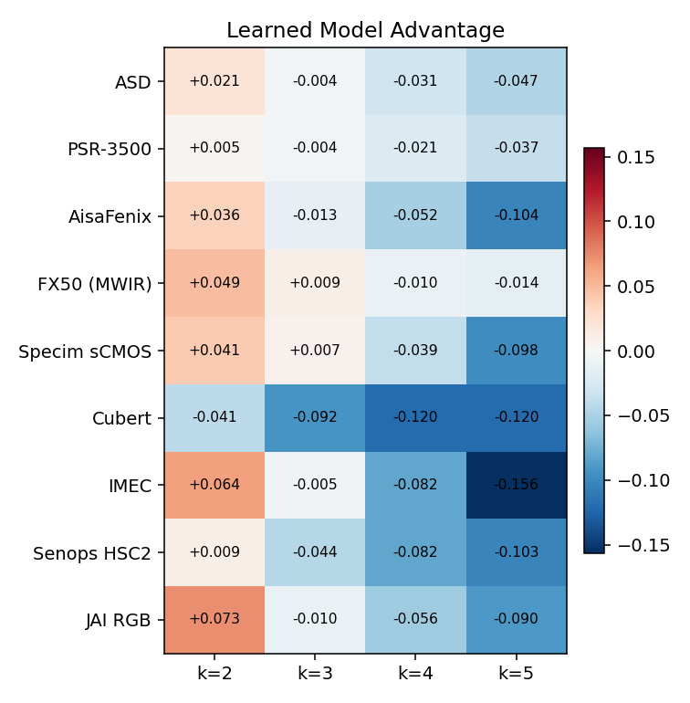
Figure 2. DL model advantage by sensor and mixture order (DL RMSE minus best-classical RMSE). Negative (blue) means the DL model is better.
The same per-sensor checkpoint is evaluated across k=2 through k=5; there is no separate model per material count. One caveat: the k=5 set is small (15 samples), so treat the quinary column as indicative, though the trend is consistent and already clear at k=3 and k=4.
Discussion
The main takeaway is not simply that the DL model wins more often at higher mixture orders. The more useful point is why that matters operationally: the model starts from pure spectra, which many teams can realistically measure and curate, rather than requiring a large labeled library of real mixtures. In many applications, collecting clean reference spectra is much easier than creating hundreds of physical mixtures with known proportions.
The mixture-order result in Table 5 and Figure 2 is also consistent with how the problem changes as samples become more complex. A two-material mixture is relatively constrained: only a few components are active, and a classical solver has fewer degrees of freedom to resolve. As more materials contribute to the same measured spectrum, the signatures overlap more, several abundance values become nonzero, and small modeling errors can spread across more components. That is where a method trained across many possible abundance combinations has more room to help.
This is the advantage of turning the pure spectral library into synthetic training data. A classical solver applies one chosen mathematical assumption directly to the measured spectrum. The DL approach can generate spectra across many material proportions, and it can be tested under different physical mixing assumptions when needed. The model is not just using the pure spectra as fixed endmembers; it is learning from a wider mixture space before being evaluated on real samples.
Classical methods still play an important role in that evaluation. FCLSU, PPNM, and MLM make different assumptions, and the strongest one differs by sensor and mixture order; in our runs no single classical solver was best everywhere, and all three won on at least one sensor. Treating "classical" as one fixed baseline would hide that variation. A useful workflow should compare the DL model against multiple classical methods, then let the data show where each approach is reliable.
This is where the Clarity platform fits naturally. Teams can import sensor data, inspect spectral signatures, manage reference libraries, generate synthetic spectra and training mixtures, train abundance models, and compare model iterations against classical methods in one workflow. As new sensors, materials, or modeling choices are added, the workflow can be repeated and modified instead of rebuilt from scratch.
Talk to engineering about your hyperspectral workflow.
Share your data, target classes, and deployment constraints so we can scope the right workflow path.
Related Resources
More product thinking and reference material from the Metaspectral team.

Metaspectral Partners with Planet to Deliver Trusted Spectral Intelligence from Tanager Hyperspectral Data
Metaspectral announced its partnership with Planet Labs PBC to deliver trusted, evidence-based spectral intelligence from Planet Tanager™ hyperspectral data through Metaspectral Clarity.
Seeing beyond the bands
Where hyperspectral analysis diverges from multispectral — and what that divergence reveals about a crop. Measured on real scenes.
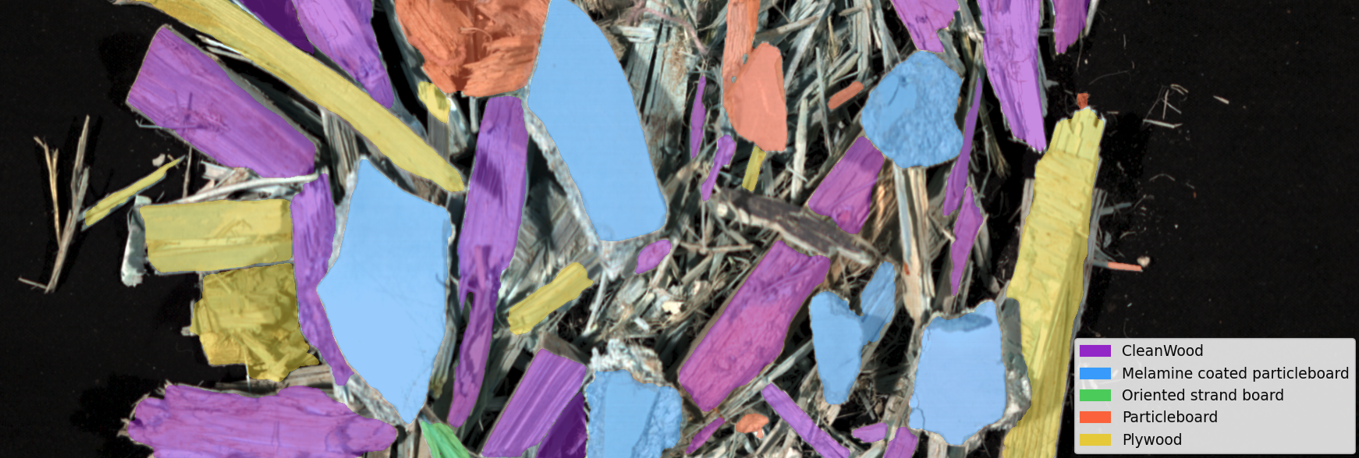
Automated Classification of Waste Wood Composites: An Evaluation of Hyperspectral Imaging and Deep Learning Pipelines
New collaborative research between UBC and Metaspectral evaluates near-infrared hyperspectral imaging and deep learning pipelines for automated classification of post-consumer waste wood composites, achieving up to 100% accuracy under controlled conditions and 91.2% on real landfill material.