From Spectral Libraries to Cuprite — Better, Faster Alteration Maps

Exploration teams looking for copper, gold, and critical-mineral deposits use hyperspectral imagery to map exposed alteration and indicator minerals—clays, micas, iron oxides, carbonates, and related assemblages. These mineral maps are interpreted alongside geology, geochemistry, geophysics, and field samples to outline alteration footprints and prioritize follow-up work; they do not directly measure buried ore or ore grade. NASA EMIT samples the surface at a nominal ground spacing of about 60 m, so one pixel commonly blends several materials. The task is therefore to identify which mineral signatures contribute to each pixel and estimate the spectral abundance of each detected mineral—the model-estimated contribution of that mineral's diagnostic spectrum, not a direct weight percentage or ore grade.

Clarity is designed to turn selected mineral spectra into sensor-ready spectral-abundance models. The workflow begins with a spectral library, adapts the model using a small number of labeled pixels from the target sensor, and then applies that model to other scenes captured by the same sensor.

The comparison below uses these names:

Term	Meaning
Clarity Model	We use Clarity BaseCNN, size medium. It maps 244-band reflectance to a 9-way softmax: eight minerals plus Background.
Training setup	Spectra are standard-normal-variate (SNV) normalized. We train with batch size 512 and dropout 0.3.
Library mix	The warm-start model is pretrained on generalized-bilinear mixtures of the eight USGS endmembers and real EMIT Background spectra. This stage does not use Tetracorder-derived mineral targets.
Scratch	The scratch model learns from Tetracorder-derived spectral-abundance targets only.
Lab→FT	Laboratory-to-fine-tune. Lab→FT starts from the library mix, then fine-tunes on the same Tetracorder-derived targets used by Scratch.

In this article we show that:

1. Clarity makes spectral-abundance maps easier to produce. Select minerals from a library (USGS, ECOSTRESS, or your own), fine-tune on a small number of labeled pixels from the same sensor, and run inference on other sites captured by that sensor. Section 1 explains the library-to-orbit gap and this workflow.
2. Our EMIT results show lower error and faster convergence. Starting from a USGS-pretrained mineral model and fine-tuning on 5%, 25%, 50%, and 100% of the labeled pixels gives lower test error than training on labeled sensor data alone, while the learning curves show that Lab→FT reaches the same validation-error levels in fewer epochs. Section 2 quantifies those results.
3. Cuprite provides the field-sample check. Using laboratory spectroscopy (LS) as the primary reference, the Clarity Model detects at least one LS-supported mineral at 10 of 12 eligible sites (83%), compared with 12 of 12 (100%) for EMIT Tetracorder. Section 3 presents the benchmark and its limits.

1. From spectral libraries to orbital maps

We start with reference spectra of known minerals. EMIT uses the USGS-developed Tetracorder system to compare these references with orbital spectra. We use its quality-filtered mineral estimates as training labels for eight minerals plus Background. These labels come from an algorithm, not field measurements, so we later check the model against laboratory results from Cuprite.

Laboratory and orbital spectra do not look identical. A laboratory spectrum represents a clean sample, while a 60 m EMIT pixel can mix minerals, soil, and vegetation. Atmospheric and lighting conditions add further differences, making mineral features weaker or blended.

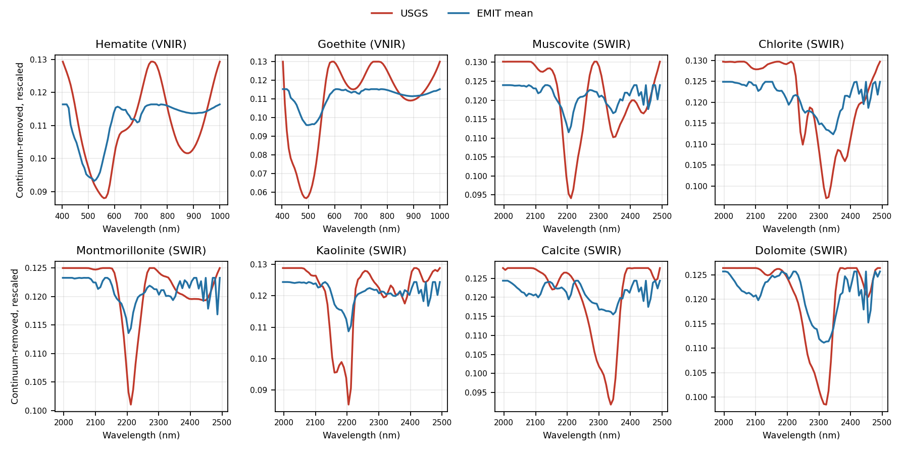
Figure 1. USGS library spectra (red) versus the mean reflectance of EMIT training pixels whose dominant Tetracorder mineral is that class (blue). For this diagnostic comparison only, each curve is continuum-removed and normalized to a common Euclidean (L2) norm. Iron oxides use VNIR (400–1000 nm); clays and carbonates use SWIR (2000–2500 nm). Table 1 reports Pearson r as a diagnostic of spectral-shape agreement, not as an abundance-accuracy score.

Mineral	Window	r vs USGS
Goethite	VNIR	0.86
Hematite	VNIR	0.66
Kaolinite	SWIR	0.85
Dolomite	SWIR	0.83
Muscovite	SWIR	0.83
Chlorite	SWIR	0.82
Calcite	SWIR	0.77
Montmorillonite	SWIR	0.75

Table 1. Pearson r between the USGS and mean EMIT spectra in Figure 1. Bold marks the lowest matches.

Across the eight minerals, r ranges from 0.66 to 0.86. Several diagnostic shapes remain well aligned, but the match is weaker for Hematite, Montmorillonite, and Calcite. The orbital spectra are also shallower and more mixed than their library counterparts. The comparison retains recognizable mineral-specific structure while leaving a measurable library-to-orbit mismatch, motivating sensor-specific adaptation rather than direct use of the clean spectra as a finished orbital model.

That leads to the question we test: Can a deep-learning model learn to predict Tetracorder-derived mineral spectral abundance directly from EMIT reflectance, and does starting from spectral-library knowledge improve that learning compared with training on Tetracorder-derived EMIT targets alone?

Building the EMIT dataset

To answer that question, we assembled 150 EMIT scenes—50 each from eastern Australia, northern Africa, and the USA. We split the data 80/20 by scene within each region, producing 120 training scenes and 30 held-out test scenes. The split is by scene rather than by pixel, so test pixels never come from a training acquisition.

Each model input contains the 244 EMIT bands retained in this dataset. Each target is a dense nine-component vector: Tetracorder-derived abundance estimates for eight minerals plus a residual Background component. The mineral estimates are quality-filtered Tetracorder outputs: Fit Score ≥ 0.46 and Band Depth Uncertainty ≤ 0.01. Undetected values are set to zero, Background is calculated as the non-negative residual after summing the eight minerals, and the resulting vector is L1-normalized. The training-ready pool contains 456,000 sampled examples.

Testing the value of library pretraining

Clarity uses the spectral library as an informed initialization, then adapts the model to the sensor. In general, the practical workflow is:

1. Select the minerals of interest from USGS, ECOSTRESS, or a user-provided library.
2. Build synthetic mixtures of those minerals with representative background spectra from the target sensor.
3. Fine-tune the library-initialized model on the labeled pixels available from the target sensor.
4. Apply the adapted model to other scenes captured by that sensor.

In the reported experiment, the library stage uses eight USGS mineral endmembers resampled to the EMIT bands and 255,285 real EMIT Background examples. Generalized bilinear mixing generates synthetic mineral–background mixtures during pretraining. Both training paths then use the same network and Tetracorder-derived target pool, isolating the effect of the library initialization.

The library warm-start is not a linear addition of USGS spectra: it uses nonlinear generalized bilinear mixing with EMIT background to better represent the scattering behavior of intimate mineral mixtures.

This design separates the two roles. The spectral library supplies mineral knowledge; the Tetracorder-derived targets teach the model how those signatures appear in EMIT pixels. Section 2 tests whether combining them lowers held-out error and reaches a given validation RMSE in fewer epochs.

2. Results on held-out EMIT scenes

We compare two models on 30 held-out scenes. Scratch uses only Tetracorder-derived targets from EMIT. Lab→FT begins with the library mixture model and then fine-tunes on the same labeled pool. Test RMSE measures agreement with held-out Tetracorder-derived spectral-abundance targets.

Tetracorder-labeled pixels	Scratch-40	Lab→FT-40
0% (library mix)	—	0.0213
5% (≈23k)	0.01077 ± 0.00006	0.00927 ± 0.00002
25% (≈114k)	0.00907 ± 0.00007	0.00829 ± 0.00005
50% (≈228k)	0.00847 ± 0.00010	0.00781 ± 0.00003
100% (≈456k)	0.00774 ± 0.00006	0.00724 ± 0.00005

Table 2. Held-out test RMSE, mean ± standard deviation across three 40-epoch runs.

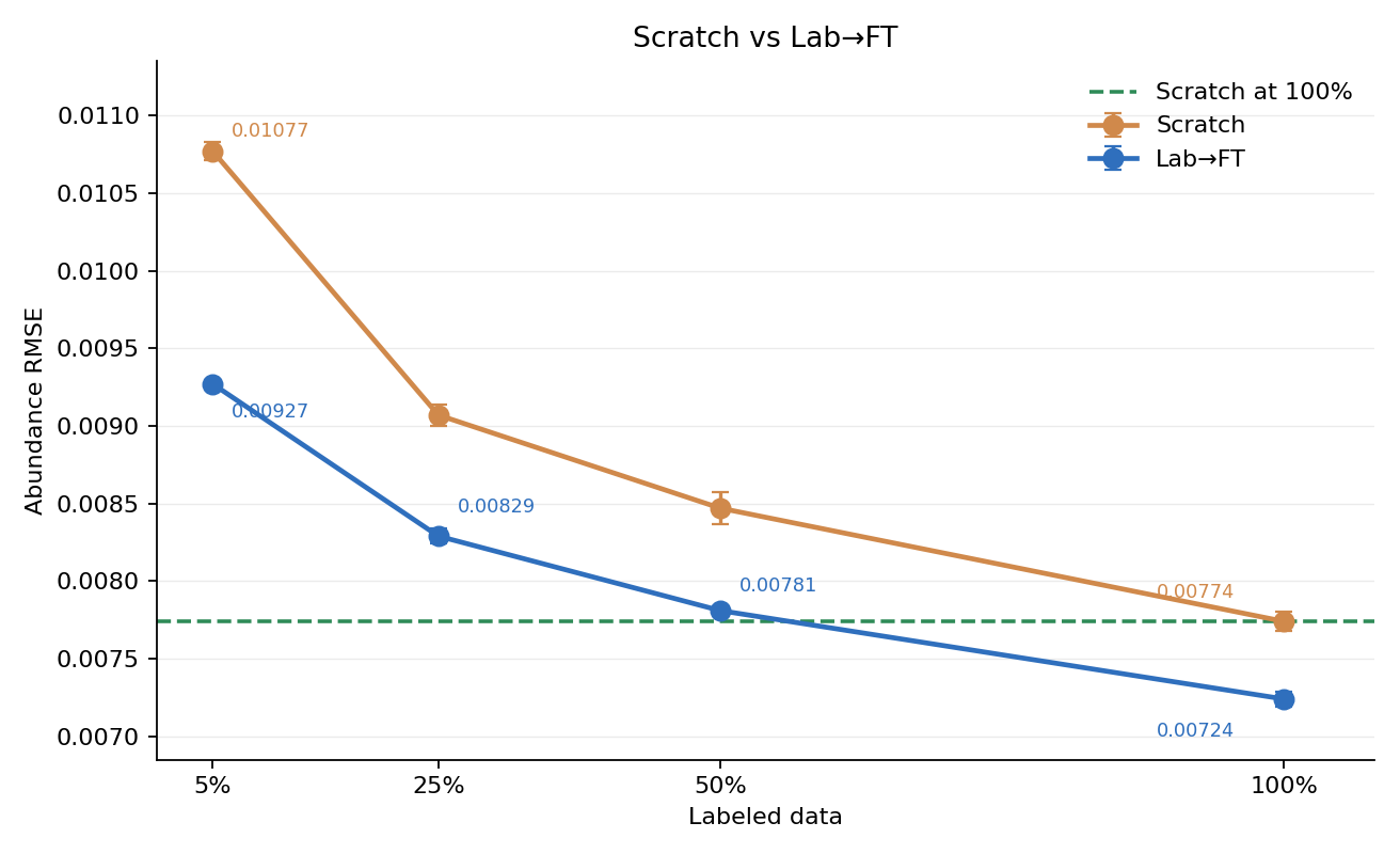
Figure 2. Mean ± standard deviation across three runs. The dashed line is scratch at 100% labeled data (0.00774).

The library initialization helps most when labels are scarce. With 5% of the labeled pixels, Lab→FT already outperforms scratch trained on the same amount of data. At 50%, Lab→FT nearly matches scratch trained on the full labeled pool. At 100%, fine-tuning remains ahead at 0.00724 versus 0.00774.

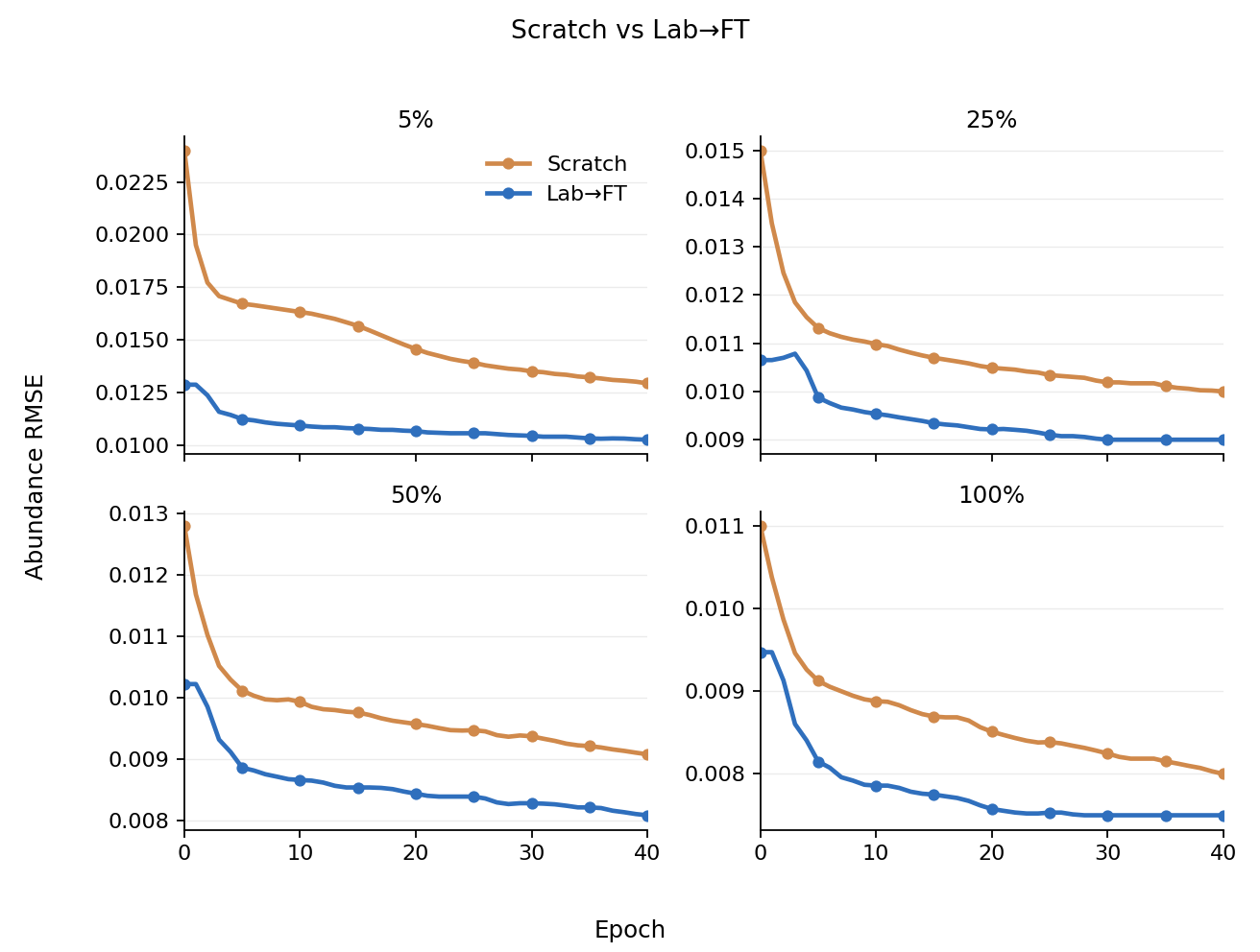
Figure 3. Validation RMSE versus epoch at 5%, 25%, 50%, and 100% labels. Lab→FT is below scratch in every panel. These curves are from one run. At 50%, Lab→FT reaches 0.0095 by epoch 4; scratch requires 24 epochs.

Lower error and faster convergence are the second result above. The library model is not a substitute for sensor labels, but it gives fine-tuning a better starting point. The result is a model that can reach a given error level with fewer labels or fewer training epochs.

These held-out results measure agreement with Tetracorder-derived targets. They show that the workflow adapts efficiently, but they do not independently establish whether the detected minerals agree with field-sample laboratory measurements. Cuprite provides that separate check.

3. Cuprite benchmark

Cuprite adds a field-sample check using the laboratory results in Table A1 of undefined. We use laboratory spectroscopy (LS) as the primary reference for spectral mineral detection. X-ray diffraction (XRD) remains a separate supporting check on crystalline minerals reported in the samples.

We use the 2023-08-04 EMIT scene, which was not included in training. At each sample location, the Clarity Model runs once on the mean reflectance spectrum of valid pixels in a 3×3 neighborhood, after the same SNV normalization used in training. EMIT Tetracorder values are averaged over the same neighborhood. Detection thresholds were fixed on validation data before testing Cuprite; the evaluation protocol defines the matching and scoring rules.

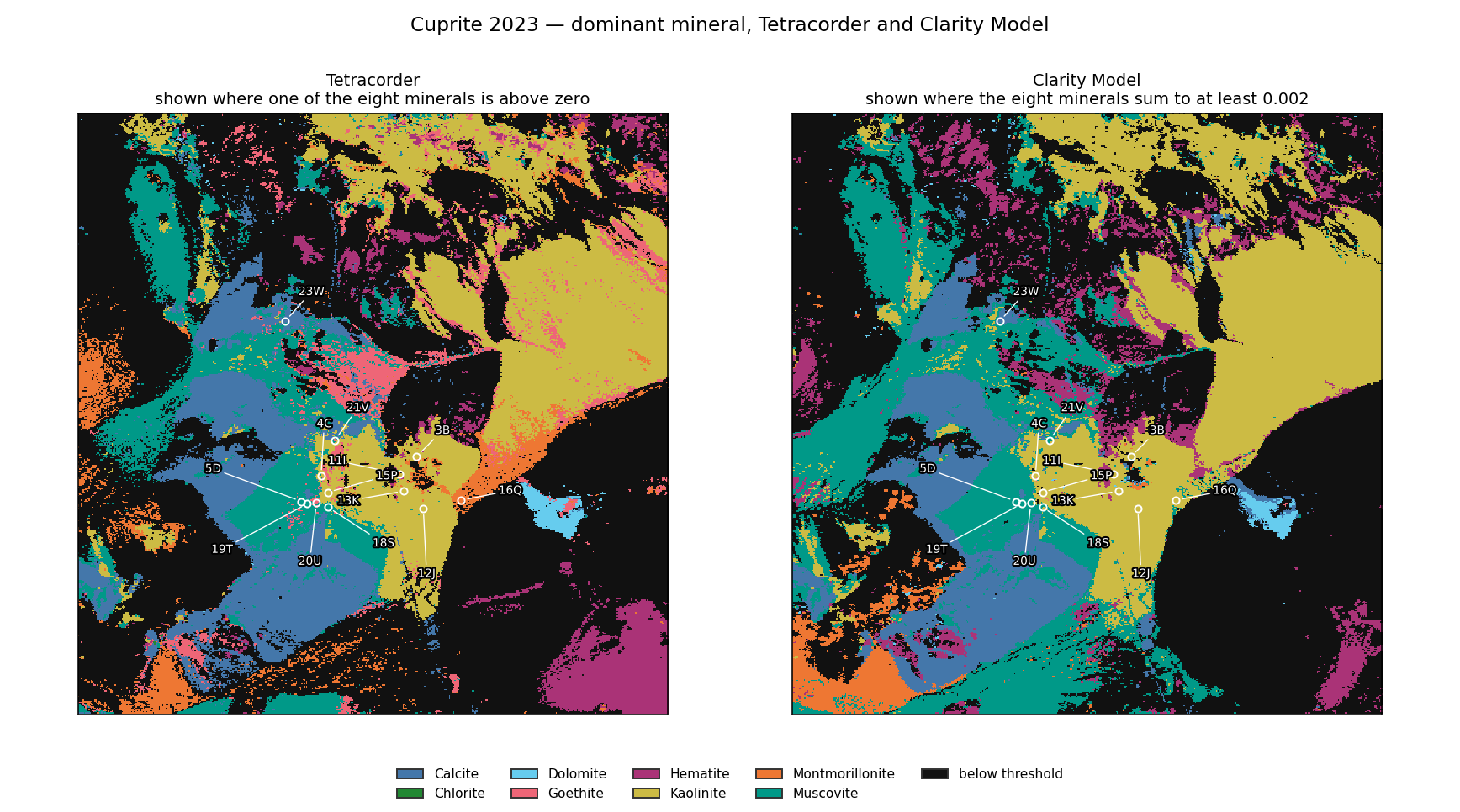
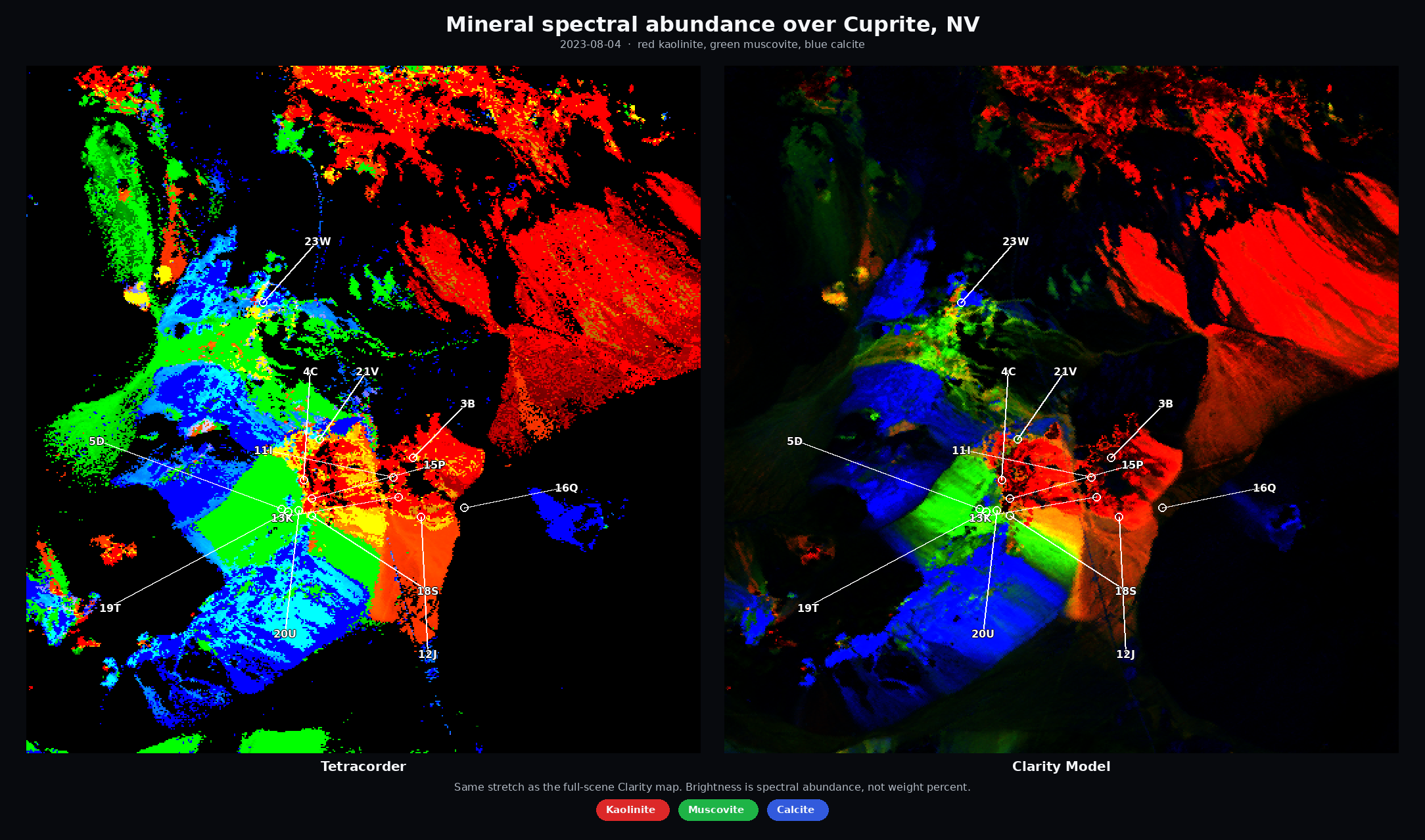
Figure 4. Dominant-mineral comparison over Cuprite on 2023-08-04. The 13 marked sites have at least one LS-reported mineral that maps to the eight model classes; 12 remain eligible for LS scoring after site 15P is excluded under the appendix protocol. For this spatial view, Tetracorder (left) is shown where one of the eight minerals is above zero; Clarity Model (right) is shown where the eight mineral outputs sum to at least 0.002, giving similar scene coverage. The 0.002 coverage display rule is not a site-scoring threshold.

Reference method	What we test	Clarity Model	EMIT Tetracorder
Laboratory spectroscopy (LS)—primary	At least one LS-listed mineral in our eight classes is detected	83% (10/12)	100% (12/12)
X-ray diffraction (XRD)—supporting	At least one XRD-listed mineral in our eight classes is detected	67% (10/15)	80% (12/15)

Table 3. Cuprite laboratory agreement. Counts are sites with at least one matching mineral / eligible sites.

Examples of the LS matches include the Clarity Model's Muscovite output matching LS white mica at 18S–21V, Kaolinite at 12J, Montmorillonite at 16Q, and Calcite at 23W. The two LS misses are 3B, where Hematite and Kaolinite remain below their thresholds, and 11I, where Montmorillonite is missed while Kaolinite and Hematite are detected.

The Cuprite result is a transfer result, not a claim that Clarity beats Tetracorder. Tetracorder detects an LS-supported mineral at all 12 eligible sites; Clarity does so at 10. The value of the benchmark is that a model adapted on other EMIT scenes produces a spatial mineral map and recovers most eligible LS-supported sites on an acquisition it never saw during training.

Discussion

The three sections answer three connected questions. First, how can a mineral library become a practical orbital mapping workflow? Clarity uses the library as an informed starting point, then adapts it to the sensor. Second, does that initialization improve model development? Across every labeled-data budget, Lab→FT lowers held-out Tetracorder-agreement error, and its learning curves reach the same validation-error levels in fewer epochs. Third, does the adapted model transfer to a recognizable field site? At Cuprite, it recovers an LS-supported mineral at 10 of 12 eligible sites on an unseen scene.

The evidence has clear boundaries. Tetracorder retains the higher Cuprite laboratory-agreement score, the Cuprite sample is small, and the site-level hit rule does not measure full-mixture recovery or penalize extra detections. The Clarity advantage is therefore the reusable workflow: select the minerals, initialize from a library, adapt with the labeled sensor pixels available, and apply the resulting model across new scenes.

Clarity supports that loop by importing EMIT-like cubes, managing mineral libraries, generating synthetic mixtures, training and comparing abundance models, and producing per-pixel maps for review.

Full supporting details—including the 23-site comparison, laboratory-name matching rules, detection thresholds, and scoring protocol—are in the Cuprite technical appendix.

---

Appendix: Cuprite site results and evaluation protocol

This appendix supports From Spectral Libraries to Cuprite — Better, Faster Alteration Maps. It contains the complete 23-site comparison, laboratory-name matching rules, detection thresholds, and site-scoring protocol.

Detailed site results

Table 4 includes all 23 published sample categories used in the comparison, including samples whose reported minerals fall outside the model's eight classes. Detections are ordered by spectral abundance within each method.

Spectral category (map code)	Sample ID	LS sample verification	XRD sample verification	Clarity Model detections ↓	EMIT Tetracorder detections ↓
Jarosite (1A)	CU91-20A	Jarosite in coating	K-jarosite in coating	None above threshold	Kaolinite 0.066; Hematite 0.022; Goethite 0.001
Hematite (3B)	CU91-223A	Hematite + Kaolinite	Disordered Hematite, Kaolinite, Quartz, Calcite, Tridymite (tr?)	None above threshold	Kaolinite 0.144; Hematite 0.010; Muscovite 0.003
Goethite (4C)	CU91-236A	Goethite, w.o. Kaolinite, Dickite	Goethite, Kaolinite, Quartz	Kaolinite 0.093; Muscovite 0.028; Goethite 0.003	Kaolinite 0.089; Muscovite 0.013; Goethite 0.003
Chlorite (5D)	CU91-238A	Chlorite + White mica	Fe-chlorite, Muscovite, Quartz, Kaolinite	Muscovite 0.169; Goethite 0.006	Muscovite 0.112; Goethite 0.004; Chlorite 0.003
Pyroxene (6E)	CU01-20A	Pyroxene + trace hydrated phases	Augite (M), Diopside (M), Anorthite (M), Forsterite (tr), Quartz (tr), Analcime (tr)	Calcite 0.021; Goethite 0.004	Calcite 0.050
K-alunite 1 (7F)	CU91-217G	K-alunite, Na/K = 0.01	K-alunite, Quartz	Kaolinite 0.074; Muscovite 0.059	Muscovite 0.079; Kaolinite 0.051; Goethite 0.003
K-alunite 2 (8G)	CU98-5C	K-alunite, Na/K = 0.07	Alunite (M), Opal-A (M), Tridymite (m), Quartz (tr)	Kaolinite 0.184	Kaolinite 0.079
Na-K±Ca alunite (9H)	CU91-217H	Multiple Alunite components	Na-alunite, Quartz	Muscovite 0.092; Kaolinite 0.058	Muscovite 0.070; Kaolinite 0.063; Goethite 0.002
Buddingtonite + Na-montmorillonite (11I)	CU91-260B	Buddingtonite + Na-montmorillonite	Buddingtonite in solid solution with K-feldspar; Quartz	Kaolinite 0.108; Hematite 0.004	Kaolinite 0.021; Montmorillonite 0.006
Well-ordered Kaolinite (12J)	CU91-200A	w.o. Kaolinite	w.o. Kaolinite, Quartz, Feldspar, Alunite	Kaolinite 0.141	Kaolinite 0.216
Disordered Kaolinite or w.o. Kaolinite ± Alunite + other (13K)	CU00-19A	Hematite; disordered Kaolinite or w.o. Kaolinite + White mica/Smectite	Clay separate: w.o. Kaolinite, Smectite (tr), Illite (tr)	Kaolinite 0.118	Kaolinite 0.108; Hematite 0.001
Dickite (14L)	CU91-219B	Dickite	Dickite, Kaolinite, Quartz, Calcite	None above threshold	Kaolinite 0.145; Goethite 0.003; Hematite 0.001
Kaolinite + White mica ± Alunite or Halloysite (15P)	CU91-242D	Trace Goethite; Halloysite or w.o. Kaolinite + White mica/Smectite	Halloysite, Quartz, Mica, Alunite, possibly Dickite	Kaolinite 0.057; Hematite 0.006	Kaolinite 0.130; Muscovite 0.009; Goethite 0.004; Hematite 0.001
Na-montmorillonite (16Q)	CU93-52	Na-montmorillonite	Quartz (M), Anorthite (m), Albite (m), Calcite (m), Orthoclase (m), Muscovite (m), Montmorillonite (m), Kaolinite (tr), Magnesiohornblende (tr)	Montmorillonite 0.017	Montmorillonite 0.054
Nontronite (17R)	CU00-13A	Nontronite	Clay separate: Smectite (M), Kaolinite (tr), Mica (tr)	None above threshold	Goethite 0.001; Hematite 0.00029
High-Al White mica 1 (18S)	CU00-5B	High-Al White mica (Al_oct = 1.845)	Quartz (M), Illite (1M and 2M2 polytypes)	Muscovite 0.071; Kaolinite 0.030	Muscovite 0.103; Goethite 0.002
Medium-high-Al White mica 2 (19T)	CU91-252D	Medium-high-Al White mica (Al_oct = 1.783)	Quartz (M), Muscovite (mostly 2M1 with trace 1M polytypes), Clinochlore (tr)	Muscovite 0.219; Goethite 0.031	Muscovite 0.154; Goethite 0.006; Chlorite 0.002
Medium-low-Al White mica 3 (20U)	CU91-250A	Medium-low-Al White mica (Al_oct = 1.707)	Quartz (M), Muscovite (2M1 and 1M polytypes)	Muscovite 0.098; Goethite 0.030	Goethite 0.118; Muscovite 0.112
Low-Al White mica 4 (21V)	CU98-8H	Low-Al White mica (Al_oct = 1.642)	Quartz (M), Muscovite (1M and 2M1 polytypes)	Muscovite 0.067	Muscovite 0.050; Kaolinite 0.021; Goethite 0.019
Calcite (23W)	CU02-11A	Calcite	Calcite (M), Quartz (tr)	Calcite 0.330	Calcite 0.332
Hydrated silica — Chalcedony and/or Opal (25X)	CU91-6A	Chalcedony	Quartz	Montmorillonite 0.014; Muscovite 0.009	Kaolinite 0.017; Montmorillonite 0.016
Opal (26Y)	CU00-15E	Opal	Cristobalite and/or Opal (M), Quartz (M), Calcite (m), Tridymite (tr)	Kaolinite 0.021; Muscovite 0.007	Kaolinite 0.022; Montmorillonite 0.012
Hydrated volcanic glass (27Z)	CU01-4A	Hydrated volcanic glass, Nontronite	Anorthite (M), Sanidine (M), Quartz (M), Cristobalite or Opal (m), Nontronite (m), Muscovite (tr), Volcanic glass	None above threshold	None

Table 4. Cuprite sample comparison. Laboratory columns and row order follow Swayze Table A1; detections are ordered by spectral abundance. Bold map codes are the 12 sites eligible for the laboratory-spectroscopy score; 15P stays in the table but is excluded from that score. M/m/tr = major/minor/trace; w.o. = well ordered.

This is a small, mixed-mineral field check—not a validation of mineral weight percentages. Field samples and the 3×3 EMIT neighborhoods cover different areas, and the predicted values are Tetracorder-style spectral abundances.

Cuprite evaluation protocol

What spectral abundance means

Spectral abundance is estimated from a mineral's absorption features in reflected light; it is not a direct measurement of the mineral's weight in the rock. As Swayze et al. (2014) explain, absorption strength also depends on grain size and mineral properties, so the strongest spectral signature need not belong to the most abundant mineral.

Here, EMIT Tetracorder supplies processed mineral spectral-abundance estimates, and the Clarity Model predicts spectral abundances learned from targets derived from those estimates. A value such as 0.066 Kaolinite does not establish 6.6% Kaolinite by weight.

Matching laboratory names

Before scoring, we translate laboratory names into the eight Clarity Model classes using Table 5. LS and XRD are matched separately; Table 4 retains their original wording.

Clarity Model class	Name in XRD or LS	Rule
Calcite	Calcite	Same name
Chlorite	Chlorite, Fe-chlorite, Clinochlore	Same group (Handbook of Mineralogy)
Dolomite	Dolomite	Same name
Goethite	Goethite	Same name
Hematite	Hematite	Same name
Kaolinite	Kaolinite, well-ordered or disordered Kaolinite	Same mineral; different ordering
Montmorillonite	Montmorillonite, Na-montmorillonite	Same mineral; sodium form
Muscovite	Muscovite, Illite, White mica	Combined Illite–Muscovite class

Table 5. Laboratory names mapped to the eight model classes; terminology follows Swayze et al. (2014).

Generic “mica” or “smectite” is too broad for an automatic match. Nontronite, Dickite, and Halloysite have no matching output class. Uncertain identifications are not treated as confirmed. Dolomite remains an output but has no laboratory reference in these samples.

Detection thresholds and site scoring

A small non-zero prediction is not automatically a detection. For each of the seven scored Clarity Model classes, a mineral must reach its minimum spectral abundance in Table 6 before it can count toward a site hit. Chlorite is excluded because its validation set is too small to support a reliable threshold.

We select each mineral's threshold by maximizing F1 against filtered Tetracorder detections on 24,000 validation pixels, taking the higher threshold on ties. All thresholds are fixed before testing Cuprite.

Clarity Model class	Detection threshold	Validation F1
Calcite	0.0162	0.837
Chlorite†	—	—
Dolomite	0.0175	0.839
Goethite	0.0024	0.775
Hematite	0.0031	0.718
Kaolinite	0.0187	0.958
Montmorillonite	0.0113	0.579
Muscovite	0.0057	0.818

Table 6. Validation-selected detection thresholds. †Chlorite is not scored because only six positive validation examples were available.

For each site, we compare Clarity Model predictions at or above their class-specific thresholds and positive, quality-filtered EMIT Tetracorder outputs with the laboratory reference. The Tetracorder data used here have already passed Fit Score ≥ 0.46 and Band Depth Uncertainty ≤ 0.01 filters. Table 5 handles differences in mineral names.

For either method, one laboratory-supported detection gives a hit; none gives a miss. We report the percentage of eligible sites with a hit, separately for LS (12 sites) and XRD (15 sites). Eligibility requires at least one laboratory-listed mineral covered by the eight classes.

Sample 15P is excluded from the LS score because its clay interpretation has alternatives, but remains visible in Table 4. XRD major/minor/trace annotations provide context rather than an abundance ranking for scoring.

This is a site-level agreement score, not full-mixture recovery or precision. One correct detection is enough, and additional unsupported detections do not reduce the score. Clarity and Tetracorder also retain their different detection rules.