Turning One Reference Spectrum Into Full-Scene Target Detection
See how a CNN-based single-spectrum detector trained on Clarity outperformed classical baselines on full-scene MUUFL target detection across multiple train-test scene pairs.

Ahmed Sigiuk
Senior Deep Learning Engineer
Using a single reference spectrum per class, a CNN-based detector trained on Clarity outperformed the strongest tested classical baseline in most object-level comparisons on the MUUFL Gulfport dataset (Multi-Unit Spectroscopic Explorer and Hyperspectral Aerial Imagery for Gulfport), an airborne hyperspectral benchmark collected over the University of Southern Mississippi Gulf Park campus in Gulfport, Mississippi.
Introduction
Hyperspectral target detection is often framed as a practical question: if you know what a target spectrum looks like, can you find that target reliably in airborne imagery? In practice, that is not as simple as matching one clean signature to one clean pixel. The MUUFL Gulfport benchmark contains 64 cloth targets in three sizes; 0.5 m × 0.5 m, 1 m × 1 m, and 3 m × 3 m, while the hyperspectral imagery is delivered at 1 m ground sample distance. That means the benchmark includes targets that are clearly subpixel, targets that are roughly pixel-sized, and targets that span multiple pixels. Many pixels are also mixed pixels, containing not only part of the target signal but also background contributions from nearby vegetation, soil, pavement, rooftops, or other materials. On top of that, the dataset explicitly includes targets that are in shadow or partially or fully occluded by trees, which makes detection even harder.
Classical detectors such as the matched filter (MF), adaptive cosine estimator (ACE), orthogonal subspace projection (OSP), and constrained energy minimization (CEM) remain strong baselines for this type of problem. But an important operational question is whether a learned model can do better when supervision is extremely sparse.
That is what we explored on the MUUFL Gulfport benchmark.
In our setup,each target class is represented by a single reference spectrum, and the task is to detect that target across cross-scene train–test pairs, where the model is trained on one flight image and evaluated on a different flight image. We evaluate three pairs shown in Table 1.. These scene pairs let us test the model across both scene changes and acquisition differences.
Our results focus on four cloth target classes: brown, dark green, pea green, and faux vineyard green. These classes provide a consistent way to compare the learned model against classical baselines across the selected scene pairs.
| Train scene | Test scene | Elevation change | Time difference between train and test scene |
| Campus 1 | Campus 3 | 3500 ft → 3500 ft | ~18 hours |
| Campus 3 | Campus 1 | 3500 ft → 3500 ft | ~18 hours |
| Campus 1 | Campus 4 | 3500 ft → 6700 ft | ~47 minutes |
| Property | Value |
| Bands | 72 |
| Wavelengths | 367.7 nm to 1043.4 nm |
| Spatial resolution | 1 m GSD |
| Target classes used here | Brown, dark green, pea green, faux vineyard green |
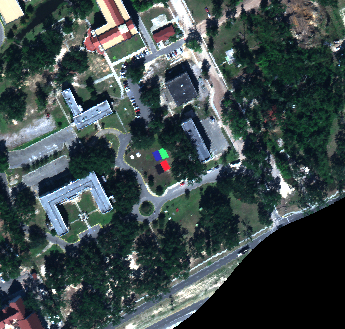
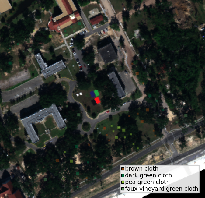
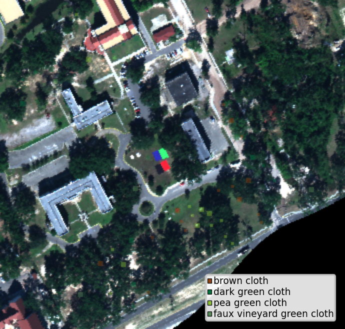
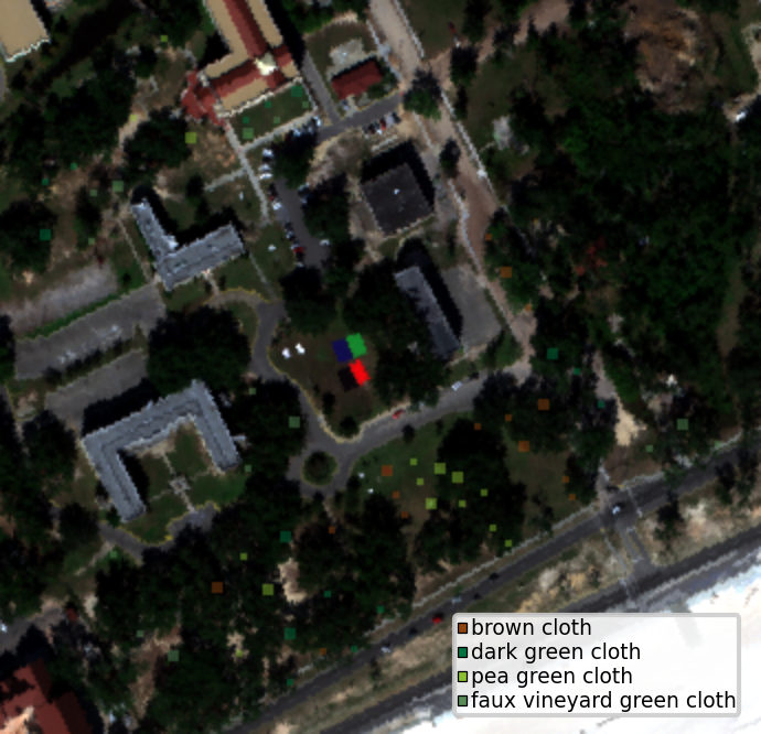
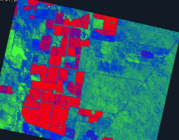
For this post, we focus on the evaluation view that is most relevant to a real scene-level detection problem: object-level detection quality under low false-alarm constraints. Figures 1 (A, B, and C) gives visual context for the three test scenes emphasized in this post.
Approach
We used a CNN spectral model trained on Clarity, Metaspectral’s hyperspectral artificial intelligence platform, for single-spectrum target detection on MUUFL. Here, “single-spectrum” means that each target class is represented by one reference spectrum, which serves as the starting point for model training. On Clarity, the training workflow expands that reference information by generating synthetic target signatures, allowing the detector to learn from a broader set of target-like examples than the original spectrum alone would provide. That matters on MUUFL because the measured image spectra are often not clean target-only signatures. Depending on target size, scene geometry, and local conditions, a pixel may contain a mixture of target and background materials, and the observed target response can also be altered by effects such as shadow or partial tree occlusion.
The model was evaluated against four classical baselines:
- MF — matched filter
- ACE — adaptive cosine estimator
- OSP — orthogonal subspace projection
- CEM — constrained energy minimization
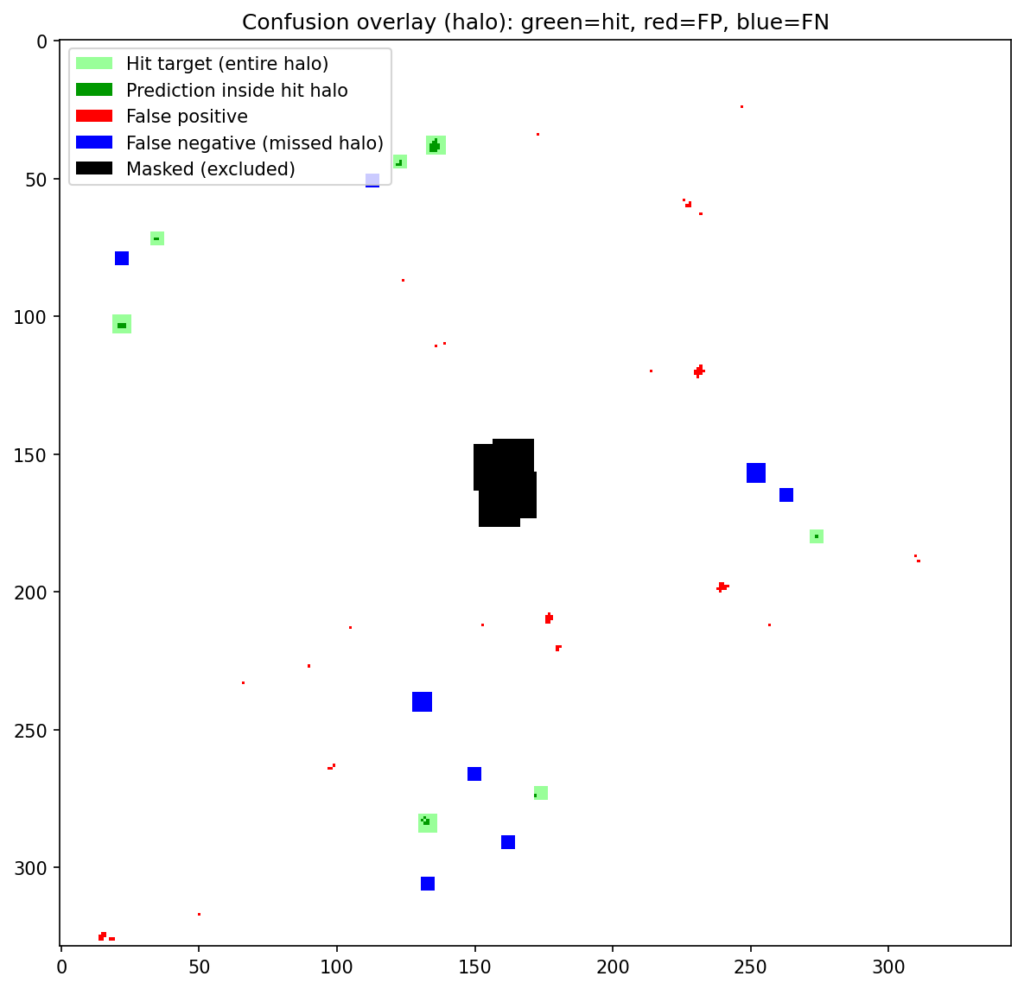
For the main result, we use object-level evaluation. Here, the model is judged as an object detector, not just as a pixel scorer. Under the Bullwinkle protocol, the model first produces a dense score map over the scene, and those scores are then converted into object-level detections. Those detections are compared with the known target locations, so performance is measured in terms of whether the detector finds the target objects while avoiding false detections elsewhere in the scene. Figure 2 shows this object-level evaluation for the same campus 1 → 3 dark green case, making the hits, false positives, and missed targets visible in the scene.
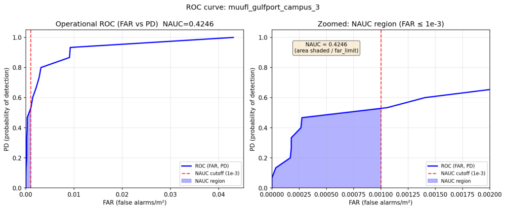
We summarize object-level detection behavior with NAUC (normalized area under the curve). In the Bullwinkle setting, this curve is an operational ROC-style curve that relates probability of detection to false alarms per square meter. Like AUROC, NAUC is threshold-independent: it summarizes performance across all decision thresholds rather than at one fixed threshold. The difference is that AUROC uses the full curve, while NAUC in this study is computed only over the low-false-alarm region up to a cutoff of 0.001 false alarms per square meter. That makes it especially useful when false positives matter, since it rewards detectors that stay strong in the operating region most relevant for practical target detection. Figure 3 shows one example of this curve for the campus 1 → 3 dark green case.
The workflow was run on Clarity end to end: hyperspectral data can be uploaded, labeled, used to train and evaluate models, and then carried forward into deployment-oriented target-detection workflows. That broader workflow is part of what makes these results meaningful beyond a single benchmark run. It makes benchmark results easier to reproduce, methods easier to compare under a consistent setup, and successful models easier to move toward deployment.
Figure 4 shows the CNN score maps before object-level post-processing or metric evaluation. Each panel corresponds to one target class and one train–test scene pair, with brighter regions indicating stronger target likelihood. These maps are useful because they show not just where the model responds, but how concentrated or diffuse those responses are across the scene. In turn, that helps explain why some class/scene combinations translate into cleaner object-level detections than others.
| campus 1 → campus 3 | campus 3 → campus 1 | campus 1 → campus 4 | |
|---|---|---|---|
| Dark Green | 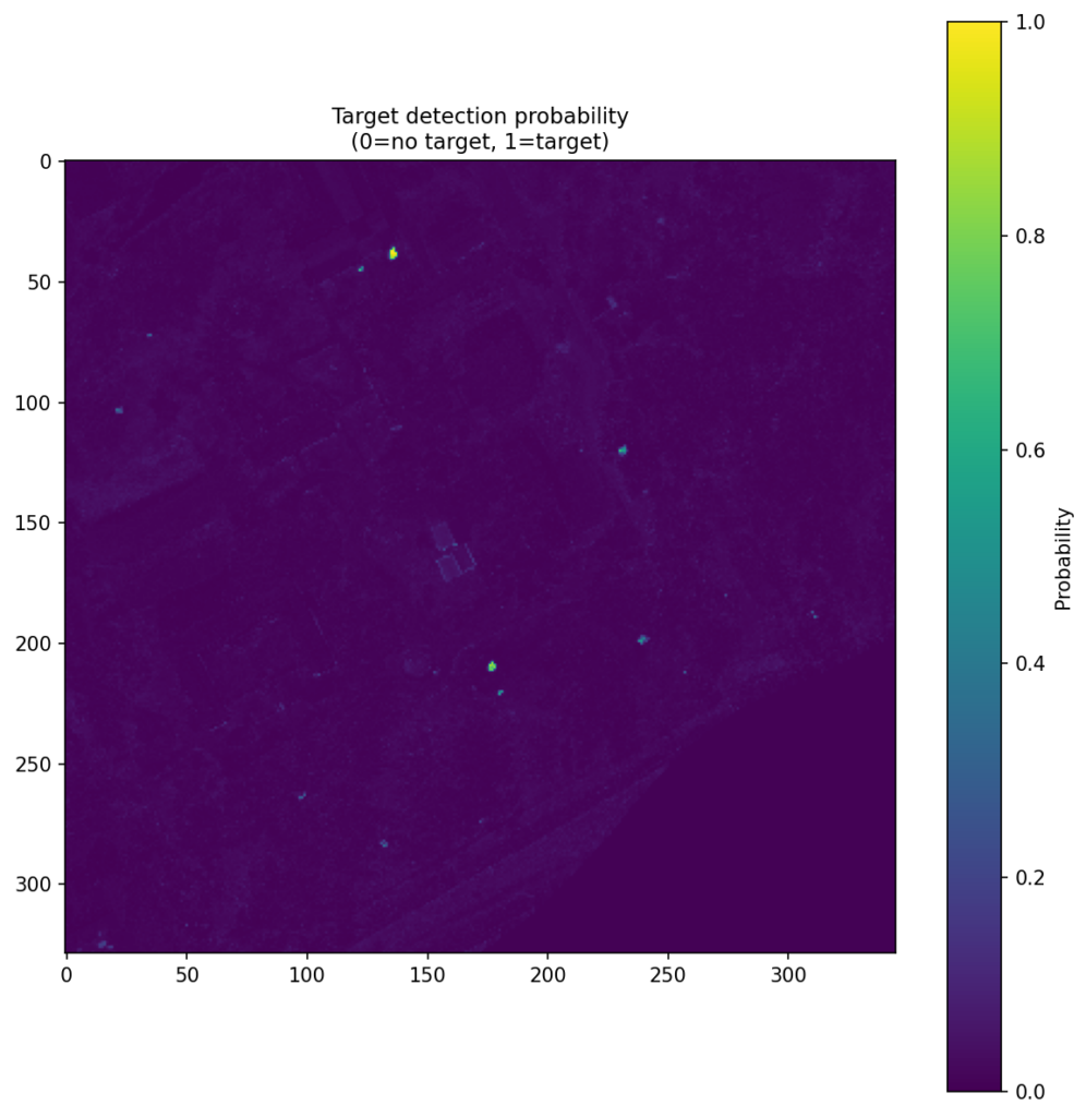 | 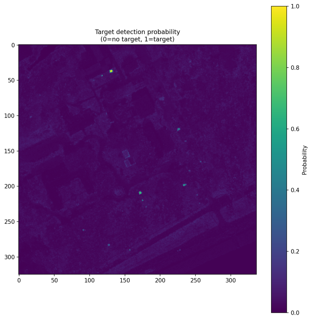 |  |
| Brown |  | 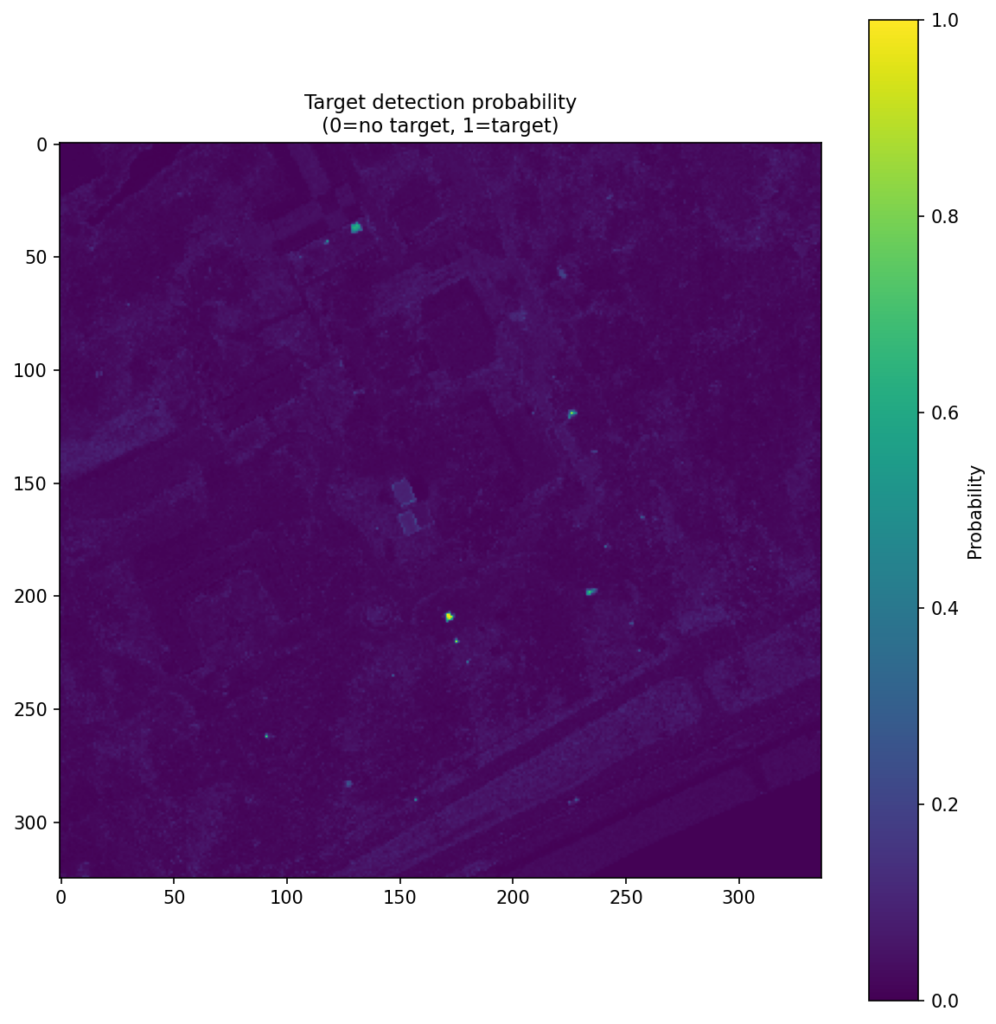 | 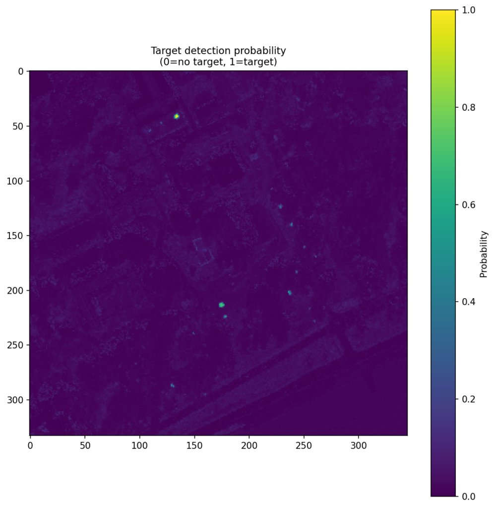 |
| Pea Green | 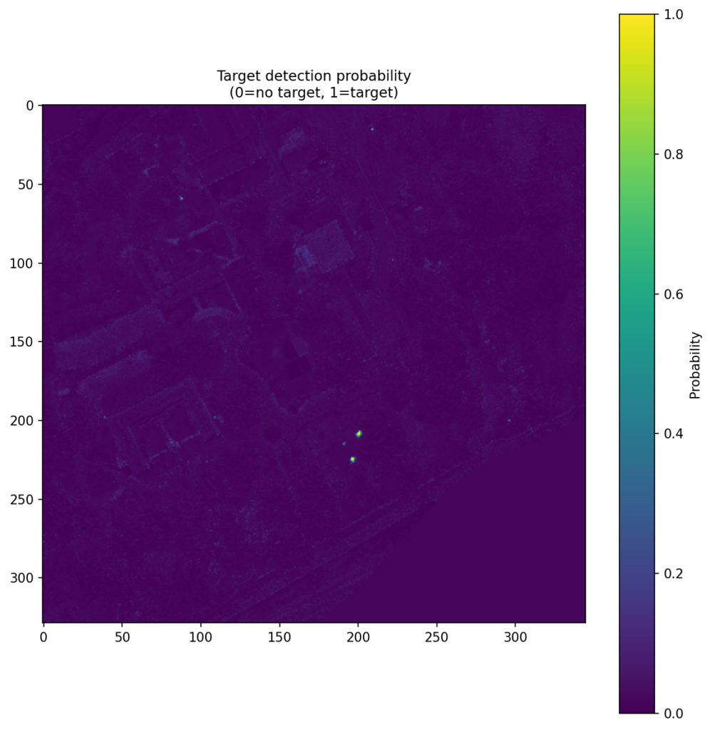 | 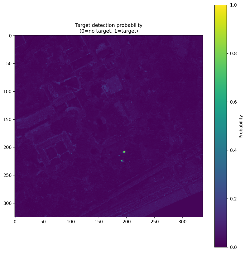 | 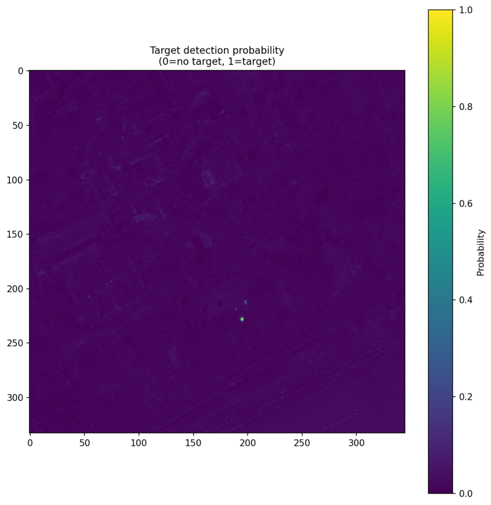 |
| Faux vineyard green | 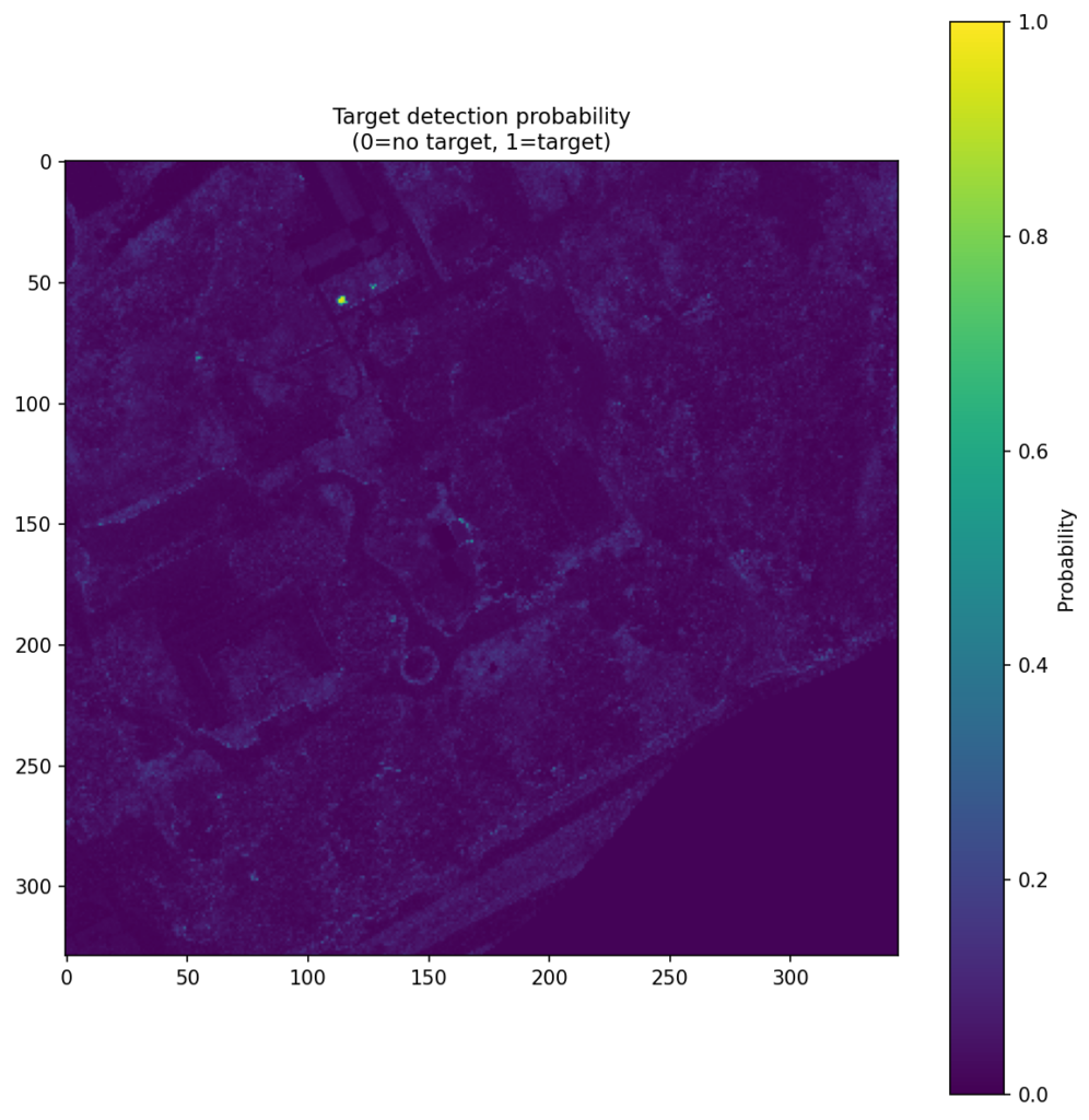 | 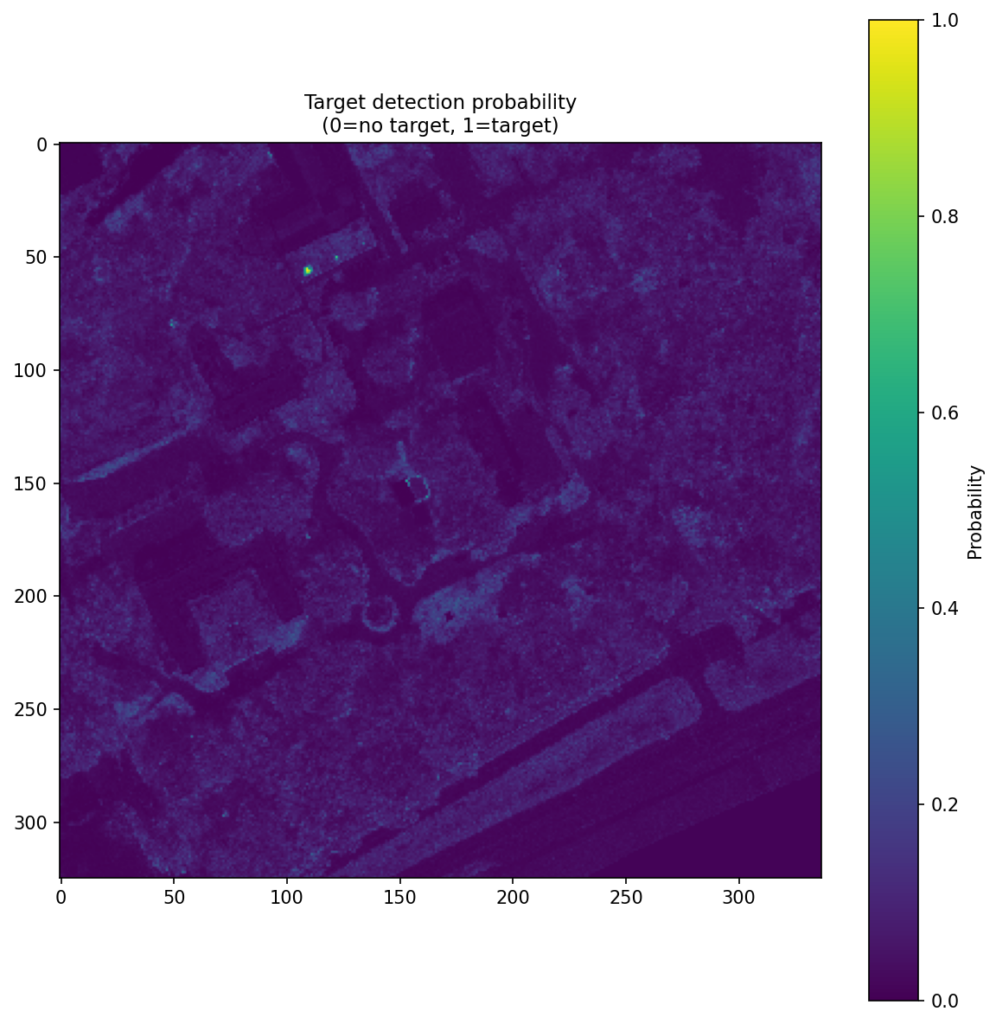 | 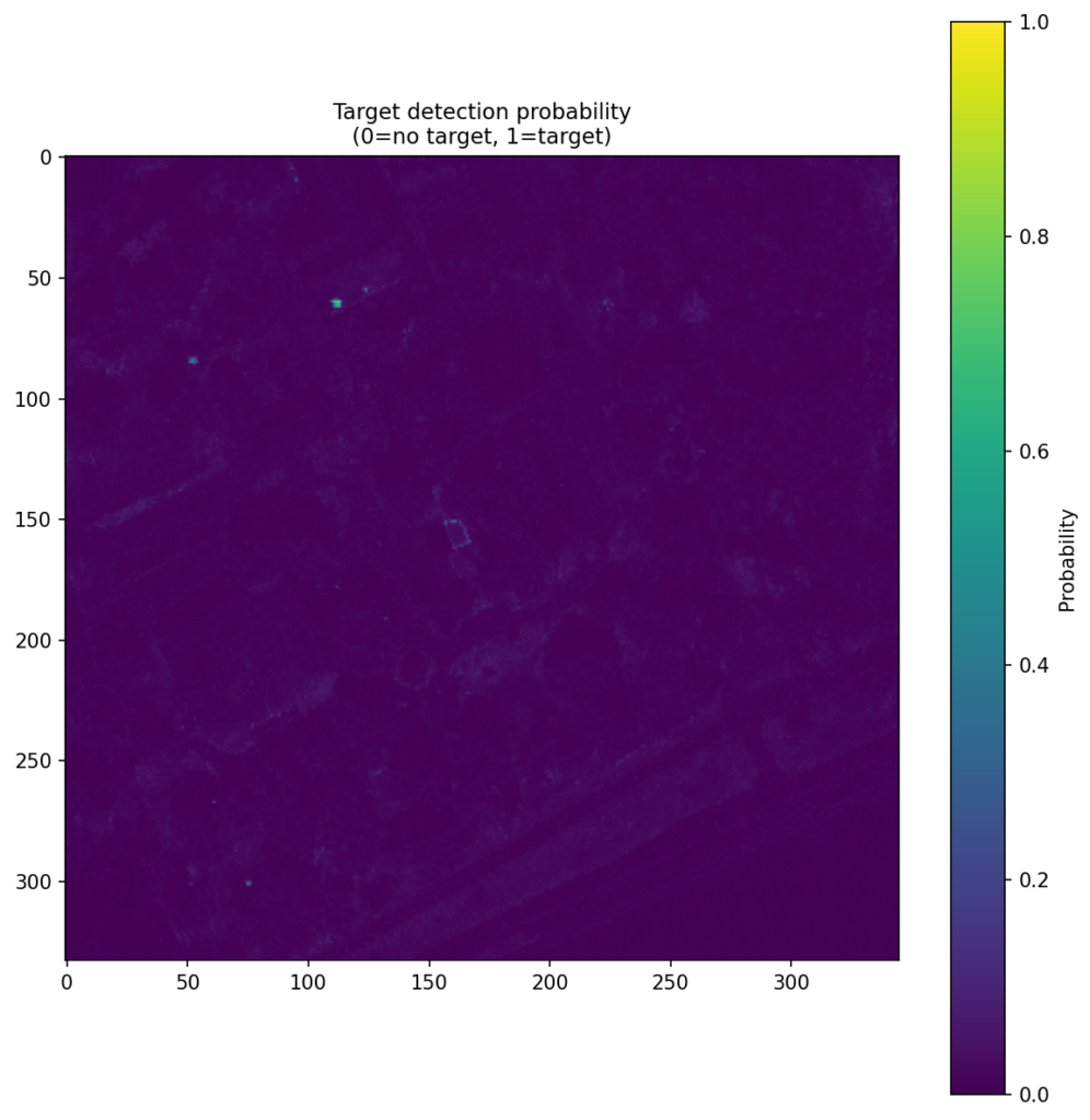 |
Key Findings
The strongest result in this study comes from the object-level evaluation described above, where the model is judged on whether its scene-level detections recover target objects while avoiding false alarms elsewhere in the image. We summarize that behavior with object-level NAUC, a normalized 0-to-1 score in which higher values indicate better low-false-alarm detection performance. Table 3 summarizes the overall outcome across all train–test scene pairs, while Table 4 (A, B and C) provides the class-by-class breakdown for each pair. Under this object-level measure, the CNN outperformed the best tested classical baseline in 9 of 12 comparisons. Here, the classical comparison is not tied to one fixed method; for each case, it refers to whichever of MF, ACE, OSP, or CEM performed best.
| Train–Test scene pair | NAUC wins |
| campus 1 → 3 | 4 / 4 |
| campus 3 → 1 | 3 / 4 |
| campus 1 → 4 | 2 / 4 |
| Overall | 9 / 12 |
Object-level results by train–test scene pair
The scene-pair comparisons make it easier to see how performance changes from one train–test setup to another.
| Class | CNN NAUC | Best classical | Classical NAUC | Δ |
| Dark green | 0.442 | MF | 0.386 | +0.056 |
| Brown | 0.512 | MF | 0.432 | +0.080 |
| Pea green | 0.310 | MF | 0.294 | +0.016 |
| Faux vineyard green | 0.564 | CEM | 0.428 | +0.136 |
In Table 4A, campus 1 → 3 train-test scene pair, the CNN is ahead in all four classes. This is the strongest and cleanest transfer result in the set.
| Class | CNN NAUC | Best classical | Classical NAUC | Δ |
| Dark green | 0.444 | ACE | 0.423 | +0.021 |
| Brown | 0.715 | ACE | 0.665 | +0.050 |
| Pea green | 0.382 | MF | 0.435 | -0.053 |
| Faux vineyard green | 0.662 | ACE | 0.613 | +0.049 |
In Table 4B, campus 3 → 1 train-test scene pair the same pattern largely holds: the CNN remains ahead in three of the four classes.
| Class | CNN NAUC | Best classical | Classical NAUC | Δ |
| Dark green | 0.401 | MF | 0.311 | +0.090 |
| Brown | 0.595 | MF | 0.561 | +0.034 |
| Pea green | 0.272 | MF | 0.310 | -0.038 |
| Faux vineyard green | 0.408 | MF | 0.432 | -0.024 |
In Table 4C, the campus 1 → 4 train–test scene pair is the toughest of the three because it introduces the largest scene and acquisition change, including a shift from the 3500 ft collection group to the 6700 ft group. This makes it the most distinct train–test pairing in the study and provides a likely explanation for the lower CNN performance: in a single-spectrum setting, larger differences in scene and acquisition conditions can make the observed target spectra less consistent with the training signatures, which in turn makes detection harder.
Discussion
The most important point in these results is not simply that a CNN outperformed several classical baselines.
The more useful point is how little information the model needed to get there.
This was a single-spectrum setup: one reference spectrum per class, applied across cross-flight train–test scene pairs. That lowers the barrier to building practical target-detection workflows. In many real Earth observation (EO) settings, assembling large, carefully curated target datasets is expensive or unrealistic. A workflow that can begin from a single target spectrum is therefore operationally attractive.
That is where the platform angle becomes important. The value here is not only the CNN itself, but the full workflow that turns a single reference spectrum into an operational target-detection pipeline. On Clarity, that starts by expanding the reference spectrum into synthetic target signatures for training. This helps because a single measured spectrum does not fully represent how a target will appear in real airborne imagery, where the observed signal can shift because of mixing, illumination, shadow, and surrounding materials. By exposing the model to a broader set of target-like examples, the workflow makes training more robust than relying on the original spectrum alone. From there, the same platform supports data upload, labeling, model training, evaluation, and deployment, making the results easier to reproduce and the path to operational use much more direct.
The results also highlight an important point about how target-detection systems should be evaluated. For this study, object-level evaluation is the most relevant measure because the task is to find target objects across the scene under false-alarm constraints. In other applications, pixel-level evaluation may be more appropriate, particularly when the emphasis is on pixel-wise target separation rather than full-scene object detection.
Conclusion
On the MUUFL Gulfport benchmark, a CNN single-spectrum detector trained on Clarity outperformed a family of classical baselines in most object-level comparisons across multiple cross-flight train–test scene pairs.
More importantly, these results show that practical hyperspectral target detection does not always require large target datasets or complex supervision. A single reference spectrum can be enough to drive a strong detection workflow when combined with a learned model and a platform that supports the full process from data ingestion through evaluation and deployment.
That is the broader takeaway from this study: the value is not only in the model, but in the ability to turn a single-spectrum detection problem into a repeatable, operational workflow.
Talk to Metaspectral about your use case.
Bring us your material stream, imagery, or operational question and we will help scope the next evaluation.
Related Resources
More product thinking and reference material from the Metaspectral team.
Seeing beyond the bands
Where hyperspectral analysis diverges from multispectral — and what that divergence reveals about a crop. Measured on real scenes.
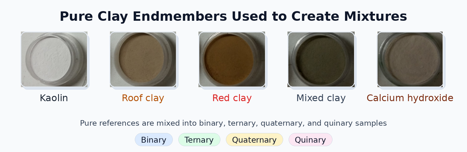
Evaluating Deep Learning Spectral Unmixing From Pure Reference Spectra
A deep learning model trained only on synthetic mixtures — generated from pure reference spectra — outperforms classical solvers on four- and five-material mixtures across nine sensors. The benchmark: 325 real clay powder mixtures measured by lab spectrometers, pushbroom cameras, snapshot cameras, MWIR, and RGB.
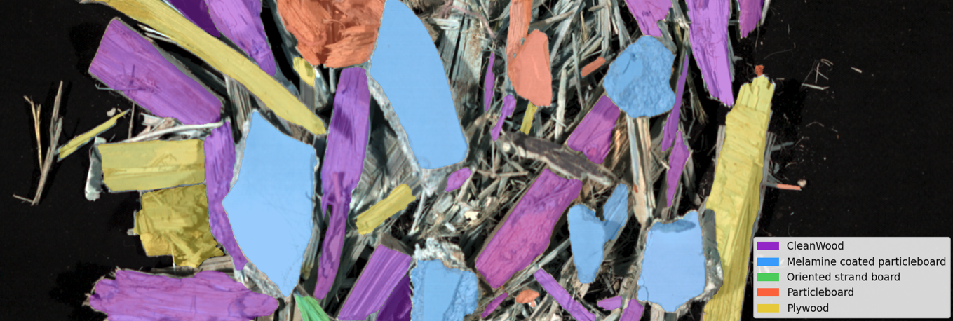
Automated Classification of Waste Wood Composites: An Evaluation of Hyperspectral Imaging and Deep Learning Pipelines
New collaborative research between UBC and Metaspectral evaluates near-infrared hyperspectral imaging and deep learning pipelines for automated classification of post-consumer waste wood composites, achieving up to 100% accuracy under controlled conditions and 91.2% on real landfill material.