Mapping Deep-Sea Manganese Nodules with Hyperspectral Imaging
A Clarity demonstration turns underwater hyperspectral imagery into seafloor maps, with promising results for distinguishing manganese nodules from sediment.

Francis Doumet
Co-Founder & CEO
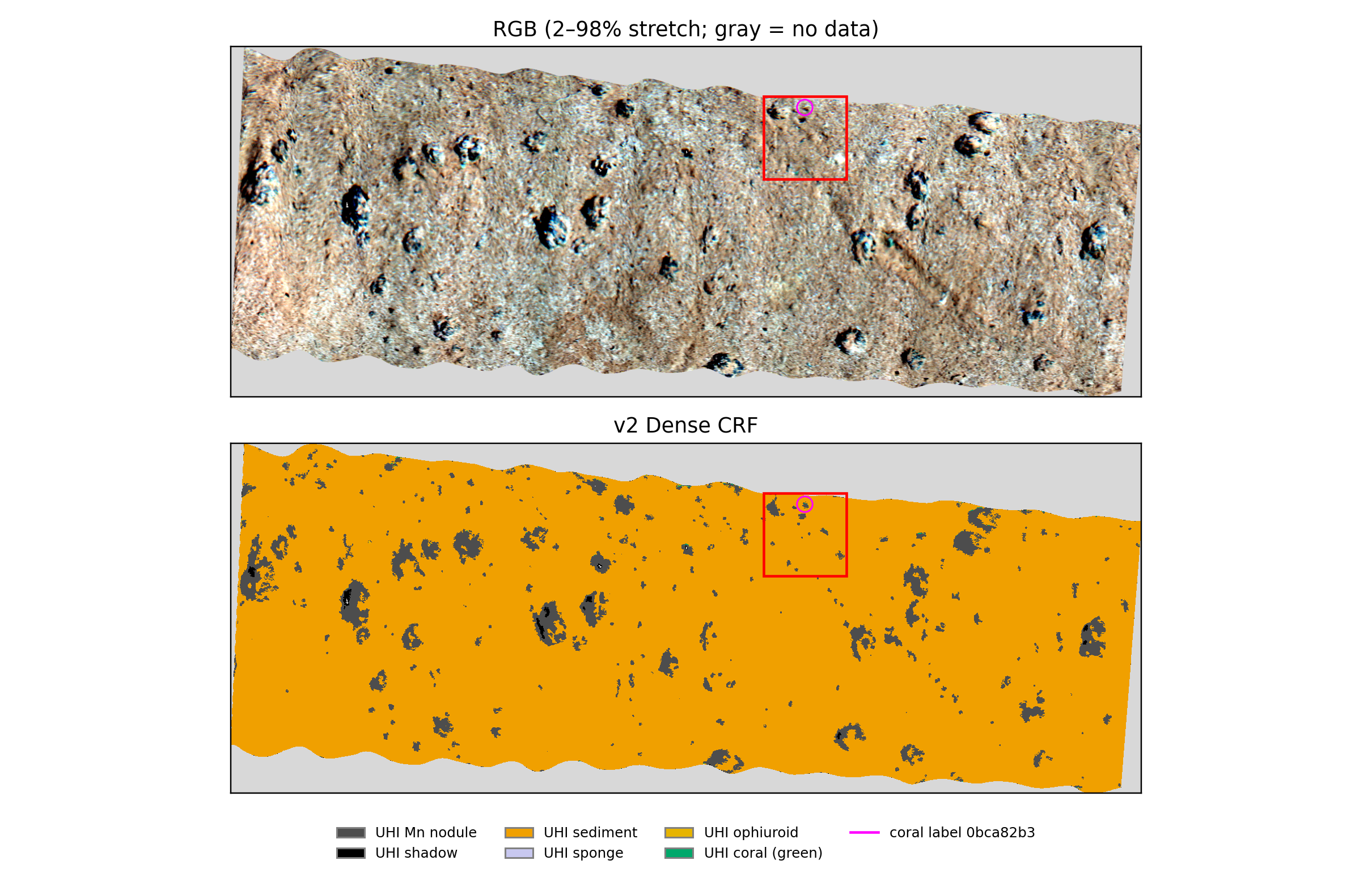
Metaspectral’s Clarity workflow mapped manganese nodules and surrounding sediment in underwater hyperspectral imagery from the Peru Basin. On a separate image kept out of training, the model achieved F1 scores of 0.93 for nodules and 0.94 for sediment against model-derived reference labels—a promising result for turning detailed seafloor imagery into interpretable maps.
Why manganese nodules matter to the mining industry
Manganese nodules are also called polymetallic nodules because they can contain several commercially important metals, including manganese, nickel, copper and cobalt. Their appeal is the possibility of recovering multiple metals from one resource. The International Seabed Authority identifies nodule abundance and combined copper, nickel and cobalt grades as important factors in assessing deposits.
Those metals serve different markets: copper is used in electrical wiring and power networks; nickel and cobalt are used in some electric-vehicle battery chemistries, as well as industrial alloys; manganese is a major steelmaking input and is also used in certain battery cathodes. This connects interest in nodules to both established industrial demand and the expansion of electrification and energy storage—not just a single battery technology.
Current market conditions highlight the importance of diversifying mineral supply. The IEA’s Global Critical Minerals Outlook 2026 reports that copper prices reached record highs during the period it reviews and projects a potential 25% copper supply deficit by 2035 based on the mine project pipeline. It also highlights a new projected cobalt supply gap following export quotas in the Democratic Republic of the Congo, alongside increasingly concentrated refining supply for minerals including nickel and manganese. These are reasons to investigate additional sources, rather than evidence that every metal faces the same shortage or that nodule extraction is automatically economic.
For mining teams evaluating nodule resources, a useful starting point is understanding where nodules occur and how much of the surveyed seafloor they cover. Hyperspectral classification can contribute that spatial picture and help focus follow-up sampling. Coverage maps complement, rather than replace, measurements of metal grade, recoverability and project economics, alongside environmental assessment and applicable approvals.
Seeing the seafloor in more detail
The imagery comes from the SO242 deep-sea survey, conducted at approximately 4,195 metres below the surface. The research described by Dumke and colleagues in 2018 explored how underwater hyperspectral imaging could map manganese-nodule fields at millimetre-scale resolution.
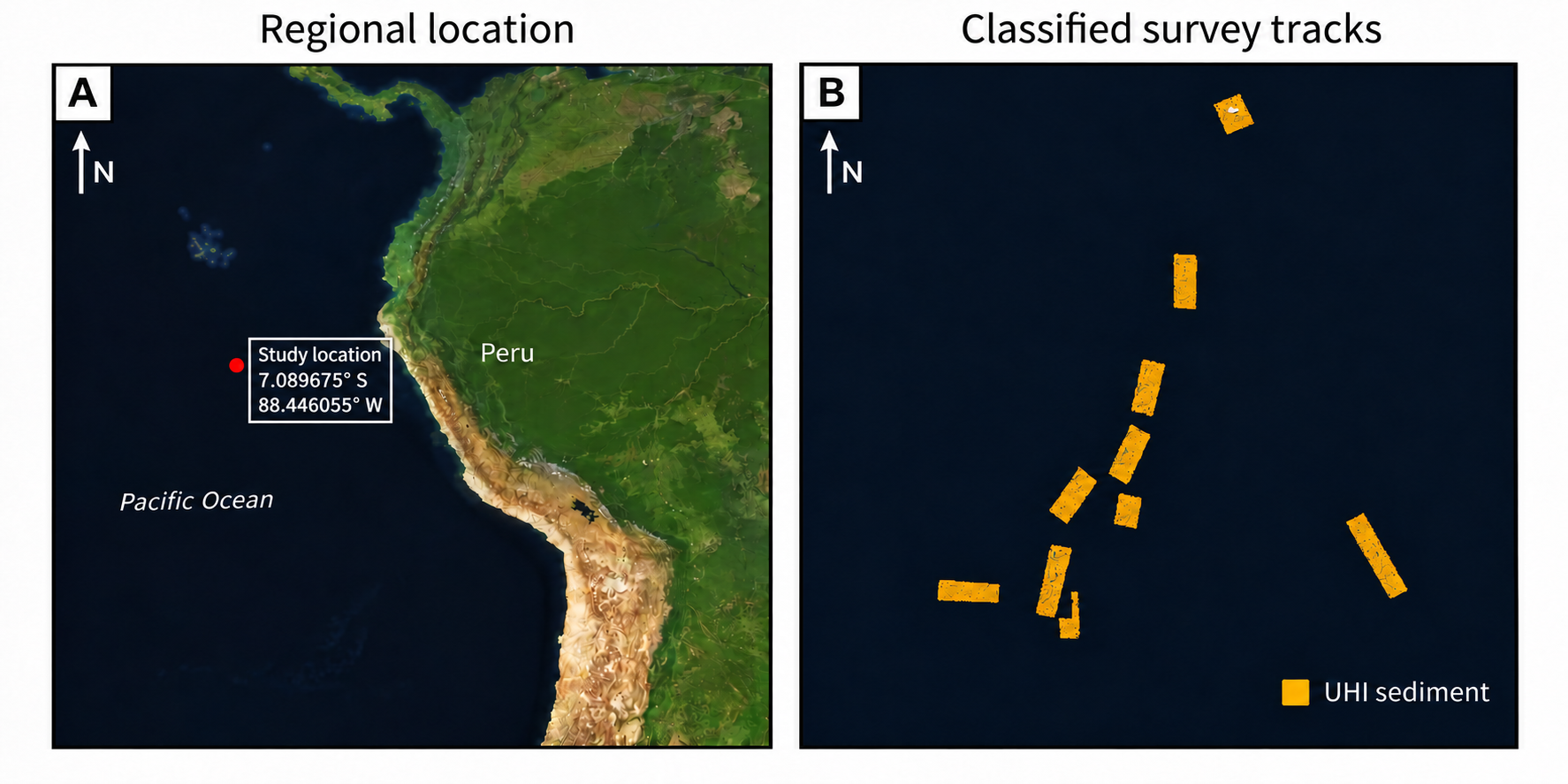
The map below places the study west of Peru in the Pacific Ocean and shows the individual survey tracks. It connects the regional setting to the narrow strips of seafloor captured by the underwater instrument: the satellite basemap provides geographic context, while the classifications come from underwater hyperspectral imagery.
Unlike a conventional colour image, hyperspectral imagery records many narrow wavelength bands. This gives a classification workflow more spectral information to work with when separating features such as nodules, sediment and small patches of marine life.
For this project, the team worked with 83-band imagery in Clarity, using a lightweight neural network to classify seafloor features. Training and validation used seven images; a separate eighth image was reserved for testing.
Strong results for nodules and sediment
The clearest result was the model’s ability to distinguish the two main materials of interest: manganese nodules and sediment. On the held-out image, the nodule F1 score was 0.93 and the sediment F1 score was 0.94.
Why the F1 score matters
A useful nodule map needs to do two things: find the nodule pixels in the reference map and avoid marking sediment as nodules. Precision asks how many pixels predicted as nodules match the nodule reference labels. Recall asks how many reference-labelled nodule pixels the model finds. F1 combines both into one score from 0 to 1, with 1 representing a perfect match. A high score therefore requires both few false detections and few missed detections.
This is especially useful when sediment occupies much more of an image than nodules: an overall accuracy figure could look impressive even if a model missed most of the nodules. Class-specific F1 makes performance on the material of interest more visible. Here, 0.93 for nodules and 0.94 for sediment indicate strong agreement with the model-derived reference labels on the held-out image; 0.93 F1 is not the same as saying “93% accurate.”
In the processed map, nodules covered approximately 6.1% of the valid scanned area. That falls within the 1–9% range reported for tracks in the original study, providing a useful contextual check.
The maps make these results tangible: areas that appear as dark nodules in the colour image correspond to nodule regions in the classification. This illustrates how a spectral analysis workflow can move beyond viewing an image to describing where different seafloor features occur.
A closer look at the marine environment
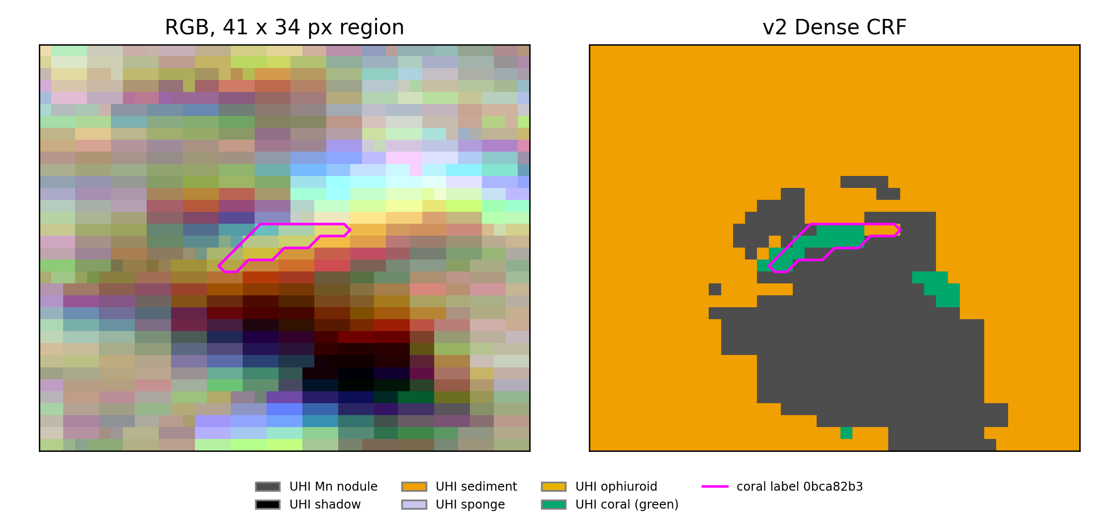
The workflow also explored classes for coral, brittle stars and sponges, alongside nodules, sediment and shadow. A 30-by-30-centimetre close-up shows how mineral features and small biological patches appear together in the same map.
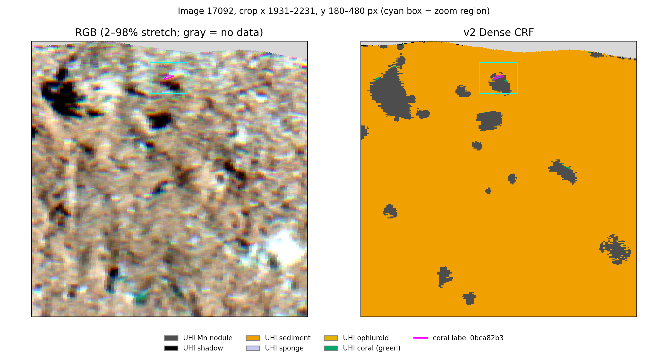
The enlarged view highlights a small coral-labelled patch near the edge of a nodule. These details show why seafloor mapping is about more than mineral coverage: the same imagery contains information about the surrounding marine environment.
From spectral data to interpretable maps
This project demonstrates a Clarity workflow for training a classifier, evaluating it on a held-out image and examining the resulting seafloor maps. The opportunity is to use the spectral detail already present in underwater imagery to build a clearer picture of nodules and their surroundings—with a defined path toward broader validation.
References
Dumke, I., et al. (2018). First hyperspectral imaging survey of the deep seafloor: High-resolution mapping of manganese nodules. Remote Sensing of Environment, 209, 19–30.
International Seabed Authority. Polymetallic Nodules.
International Energy Agency (2026). Global Critical Minerals Outlook 2026: Executive summary.
Talk to engineering about your hyperspectral workflow.
Share your data, target classes, and deployment constraints so we can scope the right workflow path.
Related Resources
More product thinking and reference material from the Metaspectral team.
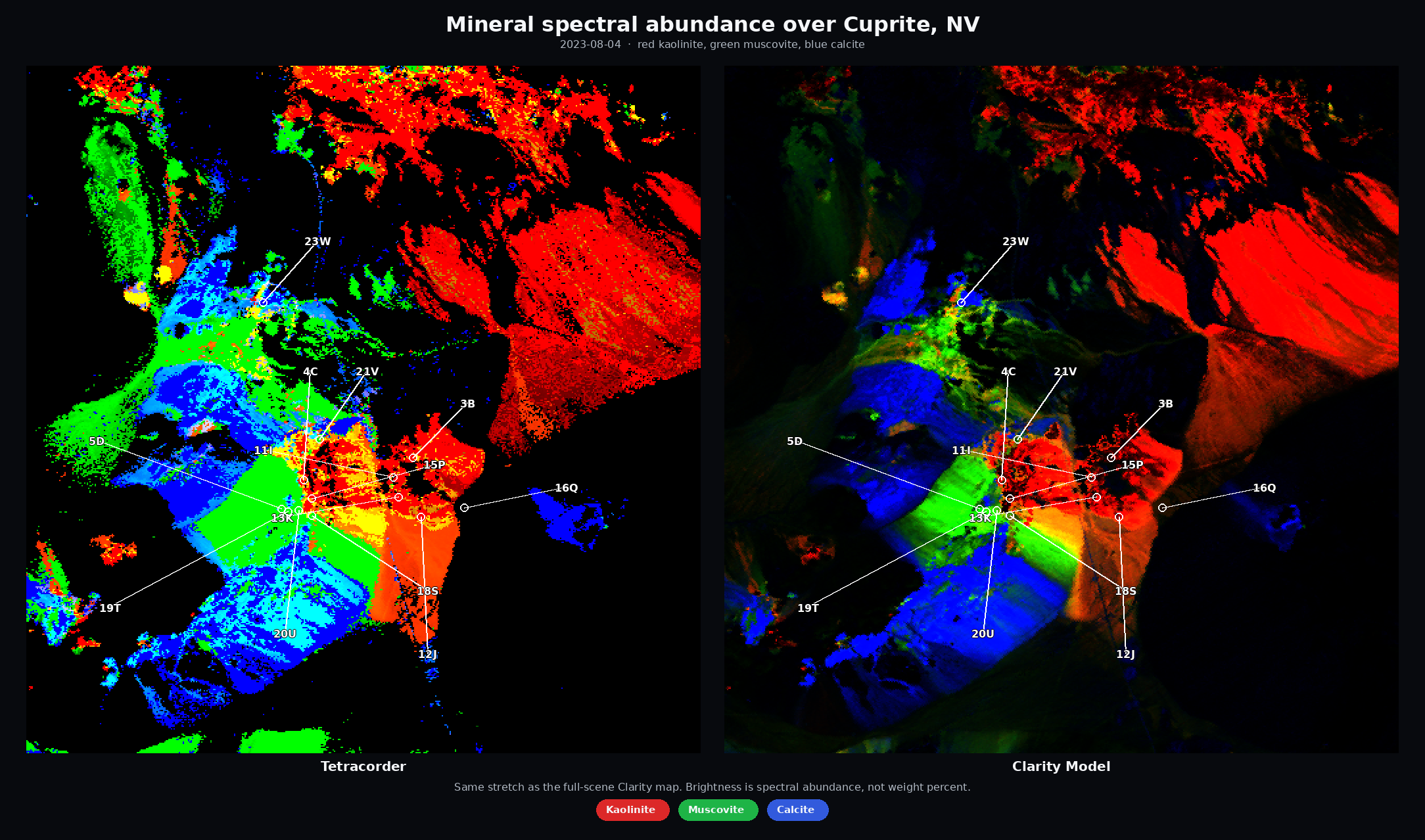
From Spectral Libraries to Cuprite — Better, Faster Alteration Maps
Exploration teams looking for copper, gold, and critical-mineral deposits use hyperspectral imagery to map exposed alteration and indicator minerals—clays, micas, iron oxides, carbonates, and related assemblages.
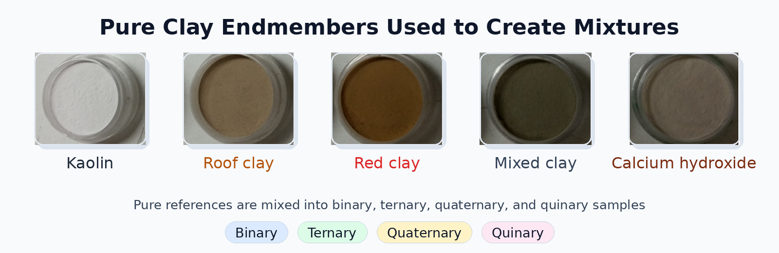
Evaluating Deep Learning Spectral Unmixing From Pure Reference Spectra
A deep learning model trained only on synthetic mixtures — generated from pure reference spectra — outperforms classical solvers on four- and five-material mixtures across nine sensors. The benchmark: 325 real clay powder mixtures measured by lab spectrometers, pushbroom cameras, snapshot cameras, MWIR, and RGB.
Seeing beyond the bands
Where hyperspectral analysis diverges from multispectral — and what that divergence reveals about a crop. Measured on real scenes.